Modelling drug-induced cellular perturbation responses with a biologically informed dual-branch transformer

Dataset preprocessing

To systematically evaluate the performance of XPert and SOTA models in drug perturbation prediction, we utilized three benchmark datasets, including two preclinical datasets—LINCS L1000 (referred to as L1000) and PANACEA—as well as one clinical dataset, namely, the cancer-drug-induced gene expression signature database (CDS-DB).

LINCS L1000 dataset

The L1000 dataset²⁴, a widely used resource for studying thousands of perturbagens in human cells, contains gene expression profiles resulting from various drug treatments across different cell lines. The LINCS L1000 data are organized into five levels at different stages of the analysis pipeline. In line with previous studies, we extracted the gene expression data of drug-induced perturbations and control samples from the L1000 level-3 data. The L1000 platform measures the mRNA transcript abundance of 978 ‘landmark’ genes, which are believed to capture approximately 80% of the information in the entire transcriptome. The transcriptional changes in these 978 genes serve as the prediction target in this study.

Data cleaning was performed to remove low-quality data, following several key steps: (1) perturbations with missing or ambiguous information were excluded; (2) profiles with low-frequency perturbation time points were removed, retaining only those with perturbation times of 3 h, 6 h or 24 h; (3) profiles that did not pass quality control were filtered out.

Subsequently, we matched each expression profile with a randomly selected dimethyl sulfoxide control sample from the same plate to create paired pre-/post-treatment profiles. Then, replicate-collapsed z-score vectors were computed to derive the unique features for each perturbation condition.

On the basis of the experimental setup, we performed further data cleaning on the L1000 dataset, resulting in several subsets, as described below. More details are provided in Supplementary Table 1:

1. (1)

   L1000_full: the complete L1000 dataset after the aforementioned cleaning process

2. (2)

   L1000_sdst: a subset retaining only the most common condition, with a perturbation dose of 10 µM and a perturbation time of 24 h

3. (3)

   L1000_mdmt: a subset that includes profiles with multiple perturbation times and doses for each cell–drug pair

4. (4)

   L1000_mdmt_pretrain: derived from L1000_full by excluding the profiles in L1000_mdmt

In particular, due to the presence of thousands of perturbation doses in the raw L1000 dataset, we grouped these doses into ten discrete dose intervals. This step was taken to facilitate standardization, unifying highly similar doses that are biologically indistinguishable (for example, 10 µM and 10.01 µM). Although such binning is advantageous for data harmonization and cross-dataset alignment, a potential limitation is that it may obscure subtle, fine-grained dose–response relationships; therefore, the choice of binning granularity should be tailored to the specific downstream task and research objective. The mapping between original doses and their corresponding dose intervals is provided in Supplementary Table 6.

PANACEA

PANACEA⁴⁴ is a resource developed by the Columbia Cancer Target Discovery and Development Center, which includes dose–response and RNA-sequencing profiles for 25 cell lines exposed to approximately 400 clinical oncology drugs. The dataset focuses on understanding tumour-specific drug MoA. It includes perturbational profiles for 32 kinase inhibitors and 11 distinct cell lines representing molecularly diverse tumour subtypes, with each perturbation performed in triplicates. The experimental conditions are standardized with each drug administered at its IC20 dose for 24 h.

For RNA-sequencing raw counts, the data are processed by calculating log₂[TPM + 1], and the final features are filtered based on the 978 landmark genes from the L1000 database. To ensure consistency, the dose of each small-molecule drug is mapped to one of the ten predefined dose ranges in the L1000 database, with the corresponding dose-to-intervals mapping provided in Supplementary Table 5. All biological replicates are averaged to generate unique profiles for each perturbation condition.

CDS-DB

CDS-DB³⁸ is a unique and comprehensive resource that provides patient-derived paired pre- and post-treatment clinical transcriptomic data. It encompasses 78 treatment-specific transcriptomic datasets, covering 85 therapeutic regimens, 39 cancer subtypes and 3,628 patient samples. The CDS-DB contains data from two different sequencing technologies—microarray and RNA-sequencing—which undergo distinct data preprocessing methods and batch effect removal procedures. To mitigate potential biases introduced by platform differences, we retained only the microarray data, which had a larger sample size.

Then, we excluded samples involving combination therapies or non-chemical drugs to maintain focus on single-agent treatments. Finally, we obtained a final dataset consisting of 613 paired profiles, representing 14 cancer subtypes and 14 different drugs. All profiles were restricted to the 978 landmark genes from the L1000 database.

Given the noteworthy variability in clinical treatment protocols, we standardized the administration dosage and treatment time into unified intervals for different therapeutic regimens. This step reduces heterogeneity in the dataset and ensures comparability across different studies. The mapping details are provided in Supplementary Tables 6 and 7.

Transcript profile embedding

Inspired by the application of transformer architectures in single-cell large language models, we adopt a similar strategy to encode gene expression profiles for pre-perturbation cells. In this context, each cell is analogous to a ‘sentence’ composed of genes, together with a special token \(< \mathrm{cls} >\) that captures the global state of each cell. Specifically, we define a transcriptomic data structure as a tensor \({X} \in {{R}}^{{N} \times ({M}+{1}) \times {d}}\), where N is the number of cells, M is the number of genes and \(d\) is the embedding dimension. For each cell i, the structure consists of two components: (1) input gene embeddings (\(\in {R}^{M\times d}\)), where each element x_{i, j} encodes the embedding of gene j in cell i, and (2) cell embedding (\(\in {R}^{1\times d}\)), represented by the \(< \mathrm{cls} >\) token. Concatenating these two parts yields the final input representation for cell i (\({C}_{i}\in {R}^{(M+1)\times d}\)), as detailed in the following subsections.

Input gene embedding

The input for gene j consists of two components: (1) gene token (\({g}_{j}\)) and (2) binned expression value (\({e}_{j}\)).

Gene tokens (\({g}_{j}\)): similar to word tokens in natural language processing⁵¹, in the XPert framework, we utilize biologically meaningful gene embeddings as gene tokens (functional representation of gene signatures). Specifically, we leverage predefined gene token embeddings from the CellLM⁵² model, which uses GraphMAE⁵³ to extract these gene embeddings from the PPI network, forming a gene vocabulary in a biologically meaningful manner. Although we focus on 978 landmark genes in this study, this method offers flexibility and can harmonize gene sets across multiple studies, enabling broad application across different datasets.

Binned expression values (\({e}_{j}\)): to address the challenges posed by variability in absolute magnitudes across different sequencing protocols, we apply a value binning technique, as proposed in scGPT¹², to convert all expression counts into relative values. For each non-zero expression value in each cell, we calculate the raw absolute values and assign them to B consecutive intervals \(\left[{b}_{k},{b}_{k+1}\right]\), where \(k\in \{1,2\ldots B\}\). Since large datasets like L1000 have already undergone transformation and batch removal steps, the bin edges are shared across all cells in the dataset, rather than varying across individual cells. However, to account for differences across datasets, bin edges should be recalculated when applying the method to new datasets. Through this binning technique, the semantic meaning of \({e}_{i}\) remains consistent across cells from different datasets.

We then introduce PyTorch embedding layers (https://pytorch.org/docs/stable/generated/torch.nn.Embedding.html) to represent the gene tokens and binned expression values, denoted as emb_g and emb_e, respectively. Each token is mapped to a fixed-length embedding vector of dimension \(d\).

The gene embedding for gene \(j\) can, thus, be expressed as

Cell embedding

In addition to the gene tokens, we introduce a special \(\bf < \mathrm{cls} >\) token to represent the overall cell state, which aggregates the learned gene-level representations during model training. The \(< \mathrm{cls} >\) token is initialized with a Gaussian distribution and is appended to the beginning of the sequence of gene tokens.

Therefore, the final input embedding for the entire cell \({C}_{i}\in {R}^{(M+1)\times d}\) is constructed by concatenating the embeddings of \(< \mathrm{cls} >\) token (C_cls) and gene tokens:

where M is the fixed number of genes for each profile.

Drug tokenization

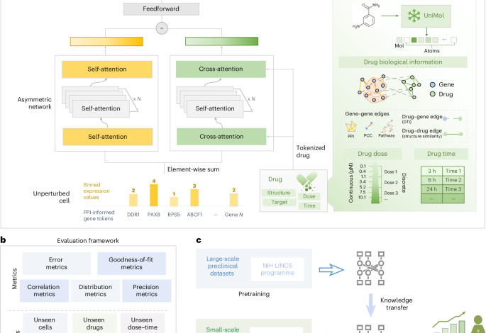
The transformer architecture requires tokenized features as input. For drugs, we consider two intrinsic features—chemical properties and biological effects—as well as additional condition tokens to represent perturbation covariates (for example, dose and time).

Chemical tokens

UniMol²¹ is a universal 3D molecular pretraining framework aimed at enhancing the representation capacity and broadening applications in drug design. It leverages a transformer-based model trained on 209 million molecular 3D conformations, outperforming SOTA methods. The model processes atom types and coordinates as inputs, using a self-attention mechanism to enable effective communication between representations, ultimately yielding robust molecular features.

Given the superiority of UniMol in representing 3D chemical structures, in the XPert architecture, we use UniMol to derive chemical tokens for each drug. Specifically, for each drug molecule, we first convert its SMILES string into canonical SMILES using the RDKit⁵⁴ package. Atom types are extracted via RDKit’s GetAtoms function as UniMol inputs. The pretrained molecular model generates a mol token (global representation) and atom tokens (local representations), both encoded as 512-dimensional vectors. These are projected onto \(d\) dimensions via a linear transformation layer. For drug \(j\), the chemical tokens form a matrix \(X\in {{{R}}}^{\left(N+1\right)\times d}\), where N denotes the preset maximum atom count (default: 120).

Although UniMol serves as the default chemical representation in XPert, we additionally evaluated the model with two alternative, widely used molecular features: Morgan Fingerprints (two-dimensional molecular descriptors, 1,024 dimensions) and KPGT molecular fingerprints (one-dimensional/two-dimensional neural fingerprints, 2,304 dimensions). Fivefold cross-validation on the L1000_sdst subset showed that XPert’s performance remained robust across different molecular features (Supplementary Table 26). This indicates that users can flexibly customize the choice of chemical representations, still fully leveraging the advantages of the XPert architecture.

Biological token based on prior-knowledge HG

There is a gap between drugs’ chemical space and their biological effect space. Chemical tokens are limited to representing features at the biological aspect. Given that DTIs are a reliable source of drug MoAs, we propose incorporating DTI information as prior knowledge to enhance the biological token representation. However, known DTIs are sparsely annotated (only 12,890 known interactions among 8,981 drugs obtained in our datasets and 19,392 proteins)^24,55. Inspired by recent studies^56,57, which constructed heterogeneous knowledge graphs to capture hidden relationships between drugs and proteins/genes, we adopt a similar methodology.

In addition to DTIs, we consider two other relationships: DDS and PPI. For DDS, we compute the Tanimoto similarity between all pairs of drugs using the RDKit package. Drug nodes with a Tanimoto similarity above 0.5 are connected, with the similarity value used as the edge weight. For PPIs, we obtain data from the STRING database²², retaining high-confidence edges (with a score greater than 700) and transforming the score \((\frac{\mathrm{score}}{1,000})\) as the edge weight. Drug nodes are initialized with UniMol \(< \mathrm{mol} >\) token embeddings, whereas protein nodes use the PPI-derived gene embeddings. To provide a clear overview of the graph structure, we report quantitative statistics of the knowledge HG, including the number of nodes, edges per relation type (DTI, DDS and PPI) and overall graph sparsity (Supplementary Table 8).

Next, we leverage a commonly used heterogeneous graph neural network model under an unsupervised contrastive learning framework to learn latent relationships between heterogeneous nodes. The heterogeneous graph neural network model consists of three HeteroConv layers constructed with SAGEConv in PyTorch Geometric, allowing message passing across different edge types. For training, we adopt a mini-batch neighbour sampling strategy to balance memory efficiency and coverage; here for each target node, a fixed number of neighbours is sampled per layer (25, 10 and 5 for the first, second and third layers, respectively). The model is optimized using Adam, with an early stopping criterion based on the validation loss. The full set of hyperparameters and training configurations is provided in Supplementary Table 9.

Positive and negative edge pairs are constructed for each relation type to enable contrastive learning, where connected pairs are treated as positives and randomly sampled non-neighbours serve as negatives. The contrastive loss was implemented following the InfoNCE formulation, with the training objective to maximize the similarity between embeddings of positive pairs and minimizing it for negative pairs.

Specifically, for each positive edge \({\left(u,v\right)}^{+}\), we sampled multiple negative pairs \({\left(u,{v}^{-}\right)}^{-}\) by replacing the target node \(v\) with non-neighbours of the source node \(u\). Let \(\mathbf{h}_{u}\) and \(\mathbf{h}_{v}\) denote the embeddings of nodes \(u\) and \(v\), respectively. The cosine similarity is scaled by a temperature parameter \(\tau\):

The probability of a positive pair being correctly identified is then

The overall loss is defined as

which encourages the embeddings of connected nodes to be close, explicitly pushing apart negative pairs.

Here N denotes the number of positive edges, \({\left(u,v\right)}^{+}\) indicates a positive node pair connected in the HG and \({\left(u,{v}^{-}\right)}^{-}\) represents negative samples obtained by randomly sampling non-neighbour nodes. \(\mathbf{h}_{u}\) and \(\mathbf{h}_{v}\) are the embedding vectors of nodes \(u\) and \(v\), respectively, and the trained model outputs \(d\)-dimensional biological token vectors for drugs.

Condition tokens

Condition tokens encode other perturbation covariates (for example, dose and time). One challenge lies in the diversity of drug dosages and protocol variability across datasets. To propose a unified tokenization strategy, we discretize raw values into predefined ranges (Supplementary Tables 5 and 6), preserving relative differences and reducing complexity. This discretization enables cross-dataset covariate normalization and mitigates scale inconsistencies. For example, preclinical and clinical doses are mapped by aligning their minimum effective ranges.

Integration of tokens

For drug \(j\), all tokens are concatenated as

For each drug, these tokens are arranged in fixed order. We then introduce learnable positional embeddings to preserve sequential relationships of each token. Using PyTorch embedding layers, positional embeddings \({E}^{\mathrm{pos}}\in {{{R}}}^{L\times d}\) (where L is the total token length) are summed in an element-wise manner with the drug tokens to produce the final input features D. Although XPert uses learnable embeddings by default, we note that fixed alternatives, such as sinusoidal positional encoding, achieve comparable performance (Supplementary Table 10).

XPert architecture overview

The XPert model is a transformer-based architecture designed to predict drug-induced transcriptional perturbations. This architecture is composed of two primary encoder branches: the base encoder branch and the Perturbation (Pert) encoder branch, designed to simultaneously encode pretreatment cellular states and drug-induced perturbation effects on gene expression.

Base encoder branch

The base encoder captures the unperturbed state of the cell by learning the dependencies between genes within the cell. It utilizes stacked self-attention layers to iteratively process the initial gene expression representation of the unperturbed cell. Given the initial representation \({C}^{\mathrm{base}}\in {{{R}}}^{\left(k+1\right)\times d}\), the encoder sequentially applies self-attention blocks across \(n\) layers:

The final output \({{C}_{n}}^{\mathrm{base}}\in {{{R}}}^{\left(k+1\right)\times d}\) represents the unperturbed cell state after \(n\) layers of self-attention.

Pert encoder branch

The Pert encoder is responsible for integrating drug molecular features with cellular context through cascaded cross-attention and self-attention layers. The cross-attention module explicitly models gene-level perturbation effects by aligning the multimodal drug representation with cellular-state features. Subsequent self-attention layers refine these interaction patterns and maintain the positional awareness of key regulatory genes.

In the cross-attention layers, the cell representation is treated as the query, and tokenized drug representation serves as the key and value matrix. This allows the model to learn gene-level perturbation effects induced by the drug. After \(m\) layers of cross-attention and self-attention, the final perturbed cell state \({{C}_{m}}^{\mathrm{pert}}\) is obtained:

Multiobjective learning

XPert uses a multiobjective learning approach, where three distinct prediction tasks are jointly optimized, including two gene-level tasks and one cell-level task.

Perturbation gene expression prediction (\({{x}}_{\mathrm{pert}}\)): the perturbation predictor is a multilayer perceptron (MLP) that uses the perturbed representation \({{C}_{n}}^{\mathrm{pert}}\) to predict the gene expression values \({x}_{\mathrm{pert}}\) after drug treatment:

The optimization objective is to minimize the mean square error (m.s.e.) loss between the ground-truth (\({x}_{\mathrm{pert}}\)) and predicted gene expression (\({\hat{x}}_{\mathrm{pert}}\)) after perturbation:

where \(\alpha\) is a weighting coefficient.

Gene expression delta prediction (x_deg): the gene expression delta predictor uses the difference between the pre-perturbation and post-perturbation gene representations \({{C}_{n}}^{\mathrm{pert}}-{{C}_{n}}^{\mathrm{base}}\) to estimate the differential gene expression values: x_deg= x_pert – x_base. Here x_deg denotes the differential gene expression vector that captures the element-wise difference between the post-perturbation expression profile x_pert and the baseline profile x_base of all the profiled genes. The loss for this task is a combination of m.s.e. and PCC losses. By incorporating the PCC loss, the model is encouraged to not only minimize the absolute differences between predictions and ground truth but also to capture the underlying correlation structure, leading to more accurate and biologically meaningful predictions.

where \(\beta\) and \(\gamma\) are weighting coefficients, and \({\hat{x}}_{{\text{deg}}}\) is the predicted differential gene expression value.

Cell-type classification: to alleviate batch effects and enhance the model’s ability to distinguish cell contexts, we introduce an auxiliary task that aims to classify the cell type based on the \(< \mathrm{cls} >\) token representations of \({{C}_{n}}^{\mathrm{pert}}\) and \({{C}_{n}}^{\mathrm{base}}\) via an added classifier. The classification task is guided by a multiclass cross-entropy loss⁵⁸:

where \({y}_{\mathrm{true}}\) represents the true cell-type labels and \({y}_{\mathrm{pred}}\) are the predicted labels; \(\delta\) is the weight of the multiclass task loss.

We further performed ablation experiments to examine the effect of individual loss components (Supplementary Note 1).

Training and testing

The training objective of XPert is to minimize the weighted sum of the losses for each task:

XPert is implemented in a PyTorch framework. For optimization, we use the Adam optimizer with an initial learning rate of 4 × 10⁻³ and a weight decay of 1 × 10⁻⁵. To facilitate more stable convergence, we use a learning rate scheduler (LambdaLR) that adjusts the learning rate dynamically. Specifically, the learning rate is reduced by a factor of 0.5 after a predetermined number of warm-up epochs. Early stopping⁵⁹ is also adopted, where training is terminated if the validation loss plateaus for 50 consecutive epochs to avoid overfitting.

Additionally, we leverage flash attention to speed up attention computation and optimize the GPU memory. This optimization is particularly advantageous for transformer-based models like XPert, especially when handling long input sequences of gene tokens, enabling seamless scalability to larger-scale gene modelling tasks.

We perform random hyperparameter search on the training set to identify the optimal combination of parameters. Supplementary Table 11 outlines the range of values and default values for each hyperparameter. The same set of hyperparameters is consistently applied across all dataset splits and datasets. On the basis of empirical evidence, usually, the default values yield satisfactory results for XPert. However, when adapting XPert to new datasets, we recommend considering larger batch sizes and more attention layers for larger datasets, reducing these parameters for smaller datasets. Additionally, experimenting with different learning rates and learning rate schedulers is advised, as XPert exhibits sensitivity to these settings.

To train and test XPert, all datasets are strictly split using fivefold cross-validation based on different perturbation attributes. A total of four split strategies are adopted:

1. (1)

   warm-start: random splitting of the dataset, with a training-to-testing ratio of 4:1 for profiles

2. (2)

   cold-drug: grouping the datasets by drug categories, with a training-to-testing ratio of 4:1 for drug types

3. (3)

   cold-cell: grouping the datasets by cell line for each profile, with a training-to-testing ratio of 4:1 for cell lines or disease types

4. (4)

   cold-dose–time: for each unique drug–cell line pair, partitioning the data based on dose–time attributes

For the L1000_sdst, PANACEA and CDS_DB datasets, the warm-start, cold-drug and cold-cell strategies are applied. For the L1000_mdmt dataset, all four split strategies are utilized.

Pretraining and fine-tuning

The pretraining step aims to equip the model with the ability to learn generalizable patterns related to cellular states, drug properties and perturbation effects using a large-scale dataset. In our setup, two datasets were used for pretraining. To assess the model’s ability to generalize across unseen dose–time conditions, we utilized the L1000_mdmt_pretrain dataset. For evaluating the model’s adaptability to independent datasets (PANACEA and CDS-DB), we used the complete L1000 dataset (L1000_mdmt_full) for pretraining. To ensure a fair comparison, all the evaluated models underwent full-parameter fine-tuning. Once pretrained, the model was fine-tuned on downstream datasets to adapt its learned representations to the specific context of the target dataset.

Implementation details

The XPert model was implemented using PyTorch (v. 2.1) as the deep learning framework. Data handling and preprocessing were performed with Scanpy. Key dependencies include torch-geometric (v. 2.6.1), torchmetrics (v. 1.6.0) and flash_attn (v. 2.6.0.post1), among others. The model was trained on an NVIDIA 4090 GPU to ensure efficient computation and faster convergence. Training on the L1000_sdst dataset took approximately 10 h, whereas the L1000_full dataset required around 60 h to fully converge.

Mean baseline models

To establish a fundamental performance benchmark and to contextualize the contributions of more complex deep learning architectures, we incorporated three mean-based baseline models. These simple yet informative baselines are designed to assess whether a model learns to predict perturbation-specific gene expression changes under multiple cell contexts beyond capturing an average expression profile, either globally or conditioned on a specific context (that is, cell line or drug).

Specifically, we considered three mean baselines:

1. (1)

   Global mean baseline (Mean): following the implementation in prior work⁶⁰, the prediction for each test sample is given by the mean expression profile across all training data, including both perturbed and control samples.

2. (2)

   Cell-specific mean baseline (Mean_cell): for a given test sample, the prediction is the average expression profile of all training samples belonging to the same cell line.

3. (3)

   Drug-specific mean baseline (Mean_drug): for a given test sample, the prediction is the average expression profile of all training samples treated with the same drug.

For the warm-start setting, all three baselines were included. For the cold-cell (cold-cancer) setting, only Mean and Mean_drug were applicable. For the cold-drug setting, only Mean and Mean_cell were used.

Evaluation metrics

To facilitate a systematic and comprehensive comparison of XPert with other SOTA models, we refer to benchmark studies such as ref. ²⁵, which evaluate performance using a variety of metrics. In this work, we consider a total of ten evaluation metrics, classified into four categories: error metrics (for example, mean squared error (m.s.e.), root mean squared error (r.m.s.e.) and mean absolute error (m.a.e.)), goodness-of-fit metrics (for example, R²), correlation metrics (for example, PCC and Spearman’s correlation (Spearman)) and distributional similarity metrics (for example, Wasserstein distance (Wasserstein) and maximum mean discrepancy (m.m.d.)). These metrics collectively provide a robust assessment of model performance in terms of prediction accuracy, statistical alignment and distributional consistency (Supplementary Table 2 lists the abbreviations of all metrics).

Error metrics

1. 1.

   m.s.e.: m.s.e. measures the average squared differences between the actual and predicted values. The formula is defined as

   $$\begin{array}{l}{\rm{m}}.{\rm{s}}.{\rm{e}}.=\frac{1}{n}\mathop{\sum }\limits_{i=1}^{n}{\left({y}_{i}-{\hat{y}}_{i}\right)}^{2}\end{array},$$

   (17)

   where \({y}_{i}\) is the actual value, \({\hat{y}}_{i}\) is the predicted value and \(n\) is the number of samples. Lower m.s.e. values indicate that the model’s predictions are closer to the true values.

   r.m.s.e.: r.m.s.e. is the square root of the m.s.e., providing a measure of prediction accuracy in the same units as the original data. It penalizes larger errors more heavily due to the squaring of differences. The formula is

   $$\begin{array}{l}\text{r.m.s.e.}=\sqrt{\frac{1}{n}{\sum }_{i=1}^{n}{\left({y}_{i}-{\hat{y}}_{{{i}}}\right)}^{2}}\end{array}.$$

   (18)

2. 2.

   m.a.e.: m.a.e. computes the average of the absolute differences between the actual and predicted values. m.a.e. provides a straightforward measure of the average magnitude of errors in the predictions. The formula is

Goodness-of-fit metrics

1. 1.

   R²: R² quantifies the proportion of variance in the dependent variable that is predictable from the independent variables, which measures how well the predicted values fit the actual data. It is a dimensionless number between 0 and 1, where higher values indicate a better fit of the model to the data. It is calculated as

where \(\bar{y}\) is the mean of the actual values.

Correlation metrics

1. 1.

   PCC: PCC measures the linear relationship between two variables. It ranges from –1 to 1, where 1 indicates a perfect positive linear correlation, –1 indicates a perfect negative linear correlation and 0 indicates no linear correlation. The formula is

   $$\begin{array}{l}\mathrm{PCC}=\frac{{\sum }_{i=1}^{n}\left({y}_{i}-\bar{y}\right)\left(\hat{{y}_{i}}-\overline{\hat{y}}\right)}{\sqrt{{\sum }_{i=1}^{n}{\left({y}_{i}-\bar{y}\right)}^{2}{\sum }_{i=1}^{n}{\left(\hat{{y}_{i}}-\overline{\hat{y}}\right)}^{2}}},\end{array}$$

   (21)

   where \(\bar{y}\) and \(\bar{\hat{y}}\) are the means of the actual and predicted values, respectively.

2. 2.

   Spearman’s rank correlation coefficient (Spearman’s \(\rho\)): Spearman evaluates the monotonic relationship between two variables by ranking the data points and computes the Pearson correlation on the ranks. It is defined as

where \({d}_{i}\) is the difference between the ranks of corresponding values \({y}_{i}\) and \({\hat{y}}_{i}\), and \(n\) is the number of samples.

Distributional similarity metrics

1. 1.

   m.m.d. quantifies the difference between two distributions based on their embeddings in a reproducing kernel Hilbert space. It is suitable for assessing distributional differences in high-dimensional spaces. The formula for m.m.d. is

   $$\begin{array}{l}{\text{m.m.d.}}^{2}={E}_{{y}_{i},{y}_{i}^{{\prime} }}\left[k\left({y}_{i},{y}_{i}^{{\prime} }\right)\right]+{E}_{{\hat{y}}_{i},{\hat{y}}_{i}^{{\prime} }}\left[k\left({\hat{y}}_{i},{\hat{y}}_{i}^{{\prime} }\right)\right]-2{E}_{{y}_{i},{\hat{y}}_{i}}\left[k\left({y}_{i},{\hat{y}}_{i}\right)\right]\end{array},$$

   (23)

   where \({y}_{i}\) and \({y}_{i}^{{\prime} }\) are samples from the actual and predicted distributions; \({\hat{y}}_{i}\) and \({\hat{y}}_{i}^{{\prime} }\) are samples from the predicted distributions. \(k\left({y}_{i},{\hat{y}}_{i}\right)\) is a kernel function, and we use the radial basis function kernel in this study. Smaller m.m.d. values indicate that the distributions of actual and predicted values are more similar.

2. 2.

   Wasserstein: the Wasserstein distance measures the difference between two probability distributions. In the context of model evaluation, it measures the ‘cost’ of transforming the predicted distribution into the actual distribution. For two probability distributions \(P\) and \(Q\), the formula is given by

where \(P\) and \(Q\) are the probability distributions of the actual and predicted values, respectively, and \(\Pi (P,Q)\) represents the set of all possible joint distributions with marginals \(P\) and \(Q\).

Precision metrics

To evaluate the model’s ability to capture differentially expressed genes (x_deg), we use precision metrics, including both positive and negative precision@K (Pos/Neg P@K), which measures the fraction of intersection between the top-K up- or downregulated genes predicted by the model and the ground truth. The formulas are as follows:

where \({G}_{K}\) represents the sets of top-K up- or downregulated genes in the ground truth and \({G\prime}_{K}\) represents the predicted top-K up- or downregulated genes. \(|\cdot |\) denotes the cardinality of a set.

UMAP and t-distributed stochastic neighbour embedding visualizations

For visualization, we first applied PCA to reduce the profile dimensionality to 40, followed by UMAP or t-distributed stochastic neighbour embedding (t-SNE) to project data into two dimensions, enabling interpretation by cell types, batch indices or other labels. For UMAP, a k-nearest-neighbour graph was constructed on principal components using k = 15 neighbours.

Statistics and reproducibility

For model performance evaluation, a paired t-test was conducted to compare the differences between XPert and baseline models under different experimental conditions. For differential gene expression analysis, a two-sample t-test was used to assess the significance of the differences between two groups (treatment versus control, response versus non-response). Detailed descriptions are provided in the figure legends. The significance level was set as ***P ≤ 0.001; 0.001 < **P ≤ 0.01; 0.01 < *P ≤ 0.05; n.s., P > 0.05.