A personalized time-resolved 3D mesh generative model for unveiling normal heart dynamics

Generative model architecture

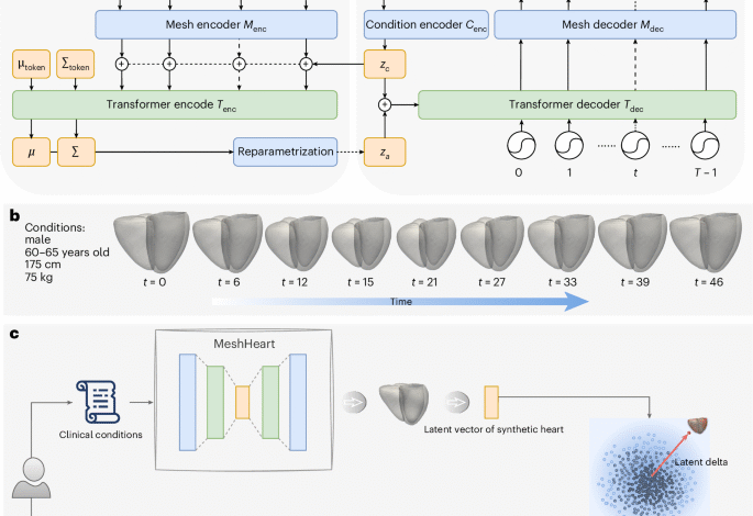
Figure 1a illustrates the architecture of the proposed generative model, MeshHeart. Given a set of clinical conditions c, our goal is to develop a model that can generate a dynamic 3D cardiac mesh sequence, X_0:T−1 = , where T denotes the number of time frames, that corresponds to the conditions c. Figure 1b shows an example of the input conditions and the generated mesh sequence. Without losing generality, we take age, sex, weight and height as conditions c in this work. Age, weight and height are continuous variables, whereas sex is a binary variable. Each cardiac mesh x_t = (v_t, e_t) is a graph with a set of vertices v and a set of edges e connecting them.

The proposed generative model consists of a mesh encoder M_enc, a transformer encoder T_enc, a condition encoder C_enc, a transformer decoder T_dec and a mesh decoder M_dec. These components are designed to work together to learn the probability distribution p_θ(x∣z_c) of the cardiac mesh sequence conditioned on clinical attributes, where θ represents the decoder parameters and z_c denotes the condition latent vector. The condition encoder C_enc, implemented as a multilayer perceptron (MLP), maps the clinical conditions c into a condition latent vector z_c.

The mesh encoder M_enc, implemented as a GCN, processes the input cardiac mesh sequence x_0:T−1. It extracts latent representations z_0:T−1, where each vector z_t corresponds to a latent representation of the cardiac mesh at time frame t. These latent vectors serve as intermediate representations of the cardiac mesh sequence.

The latent vectors z_0:T−1 from the mesh encoder are concatenated with the condition latent vector z_c to form a sequence of input tokens to the transformer encoder T_enc. The transformer encoder T_enc captures temporal dependencies across the sequence, which comprises L layers of alternating blocks of multihead self-attention (MSA) and MLP. To ensure stability and effective learning, LayerNorm (LN) is applied before each block and residual connections are applied after each block. Similar to the class token in the vision transformer⁶², we append the input tokens z_0:T−1 with two learnable parameters μ_token and Σ_token, named distribution parameter tokens, which parameterize a Gaussian distribution over the latent space. In the transformer output layer, we extract the outputs from the distribution parameter tokens as distribution parameters μ and Σ. We then use the reparameterization trick⁶³ to derive the latent z_a from μ and Σ, as shown in Fig. 1a. The encoding process is formulated as

where ~ means distributed as, indicating that the random variable ε follows a normal distribution, where the bold 1 denotes the identity matrix. The resulting latent vector z_a, derived after the reparameterization step, captures the information about the distribution of the mesh sequence. This vector is concatenated with the condition latent vector z_c to form the input to the transformer decoder T_dec. The decoder uses these concatenated vectors as keys and values in the self-attention layer, while sinusoidal temporal positional encodings⁶² serve as queries to incorporate temporal information. The temporal positional encoding p_t at time frame t is defined using the sinusoidal function with the same dimension d as z_a:

where i denotes the dimension index. The transformer decoder outputs a sequence of latent vectors, each corresponding to a mesh representation at a timepoint of the cardiac cycle. The latent vectors generated by the transformer decoder are passed through the mesh decoder M_dec, composed of fully connected (FC) layers, to reconstruct the 3D + t cardiac mesh sequence \({X}_{0:T-1}^{{\prime} }\).

Probabilistic modelling and optimization

Following the VAE formulation^63,64, we assume a prior distribution p(z_a) over the latent variable z_a. The prior p(z_a), together with the decoder (constructed by T_dec and M_dec), defines the joint distribution p(x, z_a∣z_c). To train the model and perform inference, we need to compute the posterior distribution p(z_a∣x, z_c), which is generally intractable. To turn the intractable posterior inference problem p(z_a∣x, z_c) into a tractable problem, we introduce a parametric encoder model (constructed by C_enc, M_enc and T_enc) q_ϕ(z_a∣x, z_c) with ϕ to be the variational parameters, which approximates the true but intractable posterior distribution p(z_a∣x, z_c) of the generative model, given an input x and conditions c:

where q_ϕ(z_a∣x, z_c) often adopts a simpler form, for example the Gaussian distribution^63,64. By introducing the approximate posterior q_ϕ(z_a∣x, z_c), the log-likelihood of the conditional distribution p_θ(x∣z_c) for input data x, also known as evidence, can be formulated as

where the second term denotes the KL divergence D_KL(q_ϕ∥p_θ) between q_ϕ(z_a∣x, z_c) and p_θ(z_a∣x, z_c)^63,64. It is non-negative and zero only if the approximate posterior q_ϕ(z_a∣x, z_c) equals the true posterior distribution p_θ(z_a∣x, z_c). Due to the non-negativity of the KL divergence, the first term in equation (4) is the lower bound of the evidence \(\log [{p}_{\theta }(x| {z}_{c})]\), known as the evidence lower bound (ELBO). Instead of optimizing the evidence \(\log [{p}_{\theta }(x| {z}_{c})]\), which is often intractable, we optimize the ELBO as follows:

Training loss function

Based on the ELBO, we define the concrete training loss function, which combines the mesh reconstruction loss \({{\mathcal{L}}}_{{\mathrm{R}}}\), the KL loss \({{\mathcal{L}}}_{{\mathrm{KL}}}\) and a mesh smoothing loss \({{\mathcal{L}}}_{{\mathrm{S}}}\). The mesh reconstruction loss \({{\mathcal{L}}}_{{\mathrm{R}}}\) is defined as the Chamfer distance between the reconstructed mesh sequence \({X}_{0:T-1}^{{\prime} }=({V}^{{\prime} },{E}^{{\prime} })\) and the ground truth X_0:T−1 = (V, E), formulated as \({{\mathcal{L}}}_{{\mathrm{R}}}=\frac{1}{T}\mathop{\sum }\nolimits_{t = 0}^{T-1}{D}_{{\mathrm{cham}}}({V}_{t}^{{\prime} },{V}_{t})\), where D_cham denotes the Chamber distance⁶⁵, \({V}_{t}^{{\prime} }\) and V_t denote the mesh vertex coordinates for the reconstruction and the ground truth, respectively:

In the VAE, the distribution of the latent space for z_a is encouraged to be close to a prior Gaussian distribution. The KL divergence is defined between the latent distribution and the Gaussian prior distribution. To control the trade-off between distribution fitting and diversity, we adopt the β-VAE formulation⁶⁴. The KL loss \({{\mathcal{L}}}_{{\mathrm{KL}}}\) is formulated as

which encourages the latent space \({\mathcal{N}}(\;\mu ,\Sigma )\) to be close to the prior Gaussian distribution \({\mathcal{N}}(0,{\bf{I}})\).

The Laplacian smoothing loss penalizes the difference between neighbouring vertices such as sharp changes on the mesh^66,67. It is defined as

where N_i denotes the neighbouring vertices adjacent to v_i. The total loss function L is a weighted sum of the three loss terms

In terms of implementation, the mesh encoder M_enc has three GCN layers and one FC layer. The mesh decoder M_dec is composed of five FC layers. The transformer encoder T_enc and decoder T_dec consist of two layers, four attention heads, a feed-forward size of 1,024 and a dropout rate of 0.1. The latent vector dimensions for the mesh and condition were set to 64 and 32, respectively. The model contains approximately 69.71 million parameters and was trained on an NVIDIA RTX A6000 graphics processing unit (48 GB) using the Adam optimizer with a fixed learning rate of 10⁻⁴ for 300 epochs. Training was performed with a batch size of one cardiac mesh sequence, consisting of 50 time frames. The cardiac mesh at each time frame consists of 22,043 vertices and 43,840 faces. The weights β and λ_s in the loss function were empirically set to 0.01 and 1.

Personalized normative model, latent vector and delta

MeshHeart is trained on a large population of asymptomatic hearts. Once trained, it can be used as a personalized normative model to generate a synthetic mesh sequence of a normal heart with certain attributes c, including age, sex, weight and height. For each real heart, we can then compare the real cardiac mesh sequence with the synthetic normal mesh sequence of the same attributes, to understand the deviation of the real heart from its personalized normative pattern.

To represent a cardiac mesh sequence in a low-dimensional latent space, we extract a latent vector after the transformer encoder T_enc but before the reparameterization step. The latent vector is calculated as the mean of the latent vectors at the transformer encoder output layer across 50 time frames. For calculating the latent delta, we quantify the deviation of the latent vector of the real heart to the latent vector of a group of synthetic hearts of the same attributes. Given conditions c, 100 samples of the latent variable z_a are drawn from a standard Gaussian distribution, \({z}_{a} \sim {\mathcal{N}}({\bf{0}},{\bf{I}})\), where z_a denotes the latent space after reparameterization in the VAE formulation. Each sample z_a is concatenated with the condition latent vector z_c and passed through the transformer decoder and mesh decoder to generate a synthetic cardiac mesh sequence. After synthetic mesh generation, each synthetic mesh sequence is provided to the mesh encoder M_enc and transformer encoder T_enc, to generate latent vectors across 50 time frames at the transformer output later, subsequently averaged to form the latent vector z^synth. The real heart mesh sequence is provided to the mesh encoder M_enc and transformer encoder T_enc for calculating the latent vector z^real in the same manner.

With the latent vector z^real for the real heart and the latent vector z^synth for the synthetic heart, we define the latent vector as the Euclidean distance between z^real and z^synth. As we draw 100 synthetic samples to represent a subpopulation with the same attributes, the latent delta Δz is defined as

where i denotes the sample index. The latent delta Δz provides a robust metric to evaluate individual differences in cardiac structure and motion, quantifying the deviation of the real heart from its personalized normative model.

Data and experiments

This study used a dataset of 38,309 participants obtained from the UK Biobank⁴⁶. Each participant underwent cine cardiac MR (CMR) imaging scans. From the cine CMR images, a 3D mesh sequence is derived to describe the shape and motion of the heart. The mesh sequence covers three anatomical structures, LV, Myo and RV. Each sequence contains 50 time frames over the course of a cardiac cycle. To derive cardiac meshes from the CMR images, automated segmentation⁶⁸ was applied to the images. The resulting segmentations were enhanced using an atlas-base approach⁶⁹, by registering multiple high-resolution cardiac atlases^69,70 onto the segmentations followed by label fusion, resulting in high-resolution segmentations. A 3D template mesh⁷⁰ was then fitted to the high-resolution segmentations at the ED and ES frames using non-rigid image registration, generating ED and ES cardiac meshes. Subsequently, motion tracking was performed using Deepali⁷¹, a graphics-processing-unit-accelerated version of the non-rigid registration toolbox MIRTK⁷², on cardiac segmentations across the time frames. Deformation fields were derived using a free-form deformation model with a control point spacing of [8, 8, 8]. The registration objective function included Dice similarity as the primary similarity metric and B-spline bending energy regularization with a weight of 0.01. The deformation fields were derived between time frames and applied to propagate the ED mesh and ES mesh across the cardiac cycle. The proposed meshes were averaged using weighted interpolation based on temporal proximity to ED and ES⁹ to ensure temporal smoothness of the resulting mesh sequence. All cardiac meshes maintained the same geometric structure.

The dataset was partitioned into training, validation and test sets for developing the MeshHeart model and a clinical analysis set for evaluating its performance for disease classification task. In brief, MeshHeart was trained on 15,000 healthy participants from the Cheadle imaging centre. For parameter tuning and performance evaluation, MeshHeart was evaluated on a validation set of 2,000 and a test set of 4,000 healthy participants, from three different sites, Cheadle, Reading and Newcastle centres. For clinical analysis, including performing the disease classification study and latent delta PheWAS, we used a separate set of 17,309 participants from the three imaging centres, including 7,178 healthy participants and 10,131 participants with cardiac diseases and hypertension. PheWAS was undertaken using the PheWAS R package with clinical outcomes and coded phenotypes converted to 1,163 categorical PheCodes. P values were deemed significant with Bonferroni adjustment for the number of PheCodes. The details of the dataset split and the definition of disease code are described in Supplementary Table 1.

Method comparison

To compare the generation performance of MeshHeart, we adapt three state-of-the-art generative models originally proposed for other tasks: (1) Action2Motion⁴⁷, originally developed for human motion generation; (2) actor²⁷, developed for human pose and motion generation; and (3) CHeart⁴², developed for the generation of cardiac segmentation maps, instead of cardiac meshes. We modified these models to adapt to the cardiac mesh generation task.