A process-centric manipulation taxonomy for the organization, classification and synthesis of tactile robot skills

GGTWreP framework

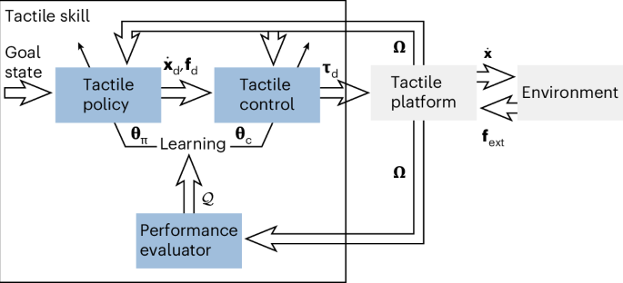
To implement process-compatible tactile skills, we rooted our efforts in the GGTWreP framework⁴¹, which has several hierarchical layers, with each layer modelling a different aspect of tactile manipulation. This multilayered structure descends from a learning layer down to the hardware system layer that is directly connected to the physical robot platform, which is coupled to the real world (Fig. 4). \({\bf{w}}\in {\mathcal{W}}\) denotes an element of the world state space \({\mathcal{W}}\), containing, for example, the robot poses, external forces or object positions. Ω denotes the percept vector, which contains information received by internal or external sensors. Appendix 1 in the Supplementary Information provides a nomenclature for all symbols used in the following.

Layers

The framework layers are described in detail in the sections below. Each layer receives inputs and extra parameters from the layer above and provides outputs to the layer below. The layers also provide constraints \({\mathbb{C}}\) in the context of the task and the limits of the system. These constraints model the limits of a valid input to the respective layer (for example, the maximum admissible velocity). The state and model estimator updates and provides the world state w with the other components based on the percept vector Ω and internal models. Figure 4 provides an overview of the GGTWreP framework with its different layers.

• The learning layer proposes parameters for the next episode in a learning process based on the parameters and quality metric of the previous episode.

• The skill state layer controls a state machine that governs the discrete behaviour of the system.

• The policy layer holds a set of (in general) ordinary differential equations embedded into a graph structure, which produce coordinated twist and wrench commands.

• The control layer implements a unified force and impedance controller that is fed by the policy layer commands and provides desired motor commands for the system layer. This layer also contains safety mechanisms to meet the system and process constraints. It also contains safety mechanisms that ensure that the system and process constraints are fulfilled.

• The system layer is the lowest layer. It sends motor commands from the control layer to the robot hardware. It provides the current robot state to the other layers.

Objects

A skill is instantiated through objects \({\mathcal{O}}\) that define the environment relevant to the skill, which is like the definition of manipulation processes introduced above. Note that all skills also contain an end effector as a default object. It has the handle EE.

Learning layer

The learning layer executes a learning algorithm that proposes a parameter candidate \({{\bf{\uptheta }}}_{i+1}\in {\mathbb{D}}\) for episode i + 1 based on the parameters θ_i and quality metric \({{\mathcal{Q}}}_{i}\) of the previous episode i and passes the candidate to the skill state layer. \({\mathbb{D}}\) is the parameter domain and is informed by the constraints \({\mathbb{C}}\). The learning layer is represented by the functional mapping:

Skill state layer

The skill state layer contains a discrete two-layered state machine that consists of four skill states: initial state s₀, policy state s_π, error state s_e and final state s₁. s₀ denotes the beginning, s₁ is active at the end, s_e represents the end state if an error occurs, and s_π activates the policy layer. Three transitions govern the switching behaviour at the top level of the state machine. They directly implement the boundary conditions from the process specification introduced above. Additionally, some of the default conditions come from the physical realities of the robot system:

• The default precondition \({{\mathcal{C}}}_{\text{pre},0}=\{{{{T}}}_{{\rm{EE}}}\in \text{ROI}\}\) states that the robot has to be within a suitable region of interest (ROI) depending on the task at hand.

• The three default error conditions \({{\mathcal{C}}}_{\text{err},0}=\{| {{\bf{f}}}_{{\rm{ext}}}| > {{\bf{f}}}_{{\rm{ext,max}}},{{{T}}}_{{\rm{EE}}}\notin \text{ROI},t > {t}_{{\rm{max}}}\}\) state that the robot may not leave the ROI, exceed the maximum external forces or exhaust the maximum time for skill execution. f_ext,max is a positive vector.

The policy state s_π contains a state machine layer known as the manipulation graph. It implements the policy state from the process specification. In this graph G(Π_g, Δ), Π_g denotes the set of policies (nodes) and Δ the set of transitions (edges). The transitions are conditions that, if true, switch the current policy according to the graph structure. The skill state layer is represented by the functional mapping:

where s is the current skill state and s_π,k the kth substate in the policy state.

Policy layer

The policy layer contains a set of ordinary differential equations Π_g. Each system represents one policy π_d and implements one process state while maintaining the stated conditions. The currently active π_d is determined by the skill state layer. The policy layer functional mapping is expressed as:

For s ≠ s_π, a default policy

is activated, where f_g denotes the current grasp force. Note that f_g,d is the desired grasp force for the end effector of the robot and is passed directly to the robot. For clarity, it was omitted from Fig. 4.

Control layer

The control layer receives commands π_d from the policy layer and calculates the desired motor commands τ_d. We chose a basic form of unified force and impedance control:

\(\tilde{{\bf{x}}}={\bf{x}}-{{\mathfrak{f}}}_\mathrm{q2a}({{\bf{x}}}_\mathrm{d})\) denotes the motion error and \({{\mathfrak{f}}}_\mathrm{q2a}\) is a transformation from quaternion to axis-angle representation. K_d is the desired positive definite stiffness matrix, D_d is the desired positive definite damping, and θ_c,d and θ_c,k are the damping factors and stiffness gains. M_x(q) denotes the Cartesian mass matrix³⁷.

Architecturally, the control layer is encoded by the functional mapping

Furthermore, the control layer hosts safety mechanisms such as value and rate limitations, collision detection, reflexes and virtual walls.

System layer

The system layer is expressed by the functional mapping

It defines the control/sensing interface for the hardware system and other devices in the robot and encapsulates any subsequent hardware-specific control loops.

State and model estimator

The state and model estimator holds all the models for internal and external processes. Examples of internal models are the estimated mass matrix \(\hat{{{M}}}({\bf{q}})\), Coriolis forces \(\hat{{\bf{C}}}({\bf{q}},\dot{{\bf{q}}})\) and gravity vector \(\hat{{\bf{g}}}({\bf{q}})\). External models describe the state of environmental elements, such as the physical objects handled by the robot. For example, if the robot were to place an object at a new location, a model of the object would be updated with the new pose. The estimator continuously updates the models using Ω. Its functional mapping is

Task frame

The task frame T defines a coordinate frame ^OT_T relative to the origin frame of the robot O. π_d is then calculated in the task frame and transformed through ^OT_T into the frame of the origin.

Implementation example

In this section, the steps from a process to a skill implementation is outlined for the two process examples inserting an Ethernet plug and cutting a piece of cloth. The details of the policy selection through \({\mathcal{T}}\) can be found in appendix 6 in the Supplementary Information together with a visualization in Supplementary Fig. 1.

Inserting an Ethernet plug

In general, an insertion process involves fitting one object into another by aligning their geometries to achieve a form fit. In an industrial context, this process is essential for tasks such as part-mating. Process experts may use specialized literature, such as ref. ⁵⁰ and norms⁵¹, which is a source of process constraints and requirements, such as maximum forces, velocities and so on. In the GGTWreP framework, these constraints can be directly represented as \({{\mathbb{C}}}_\mathrm{s}\), \({{\mathbb{C}}}_{\uppi }\), \({{\mathbb{C}}}_\mathrm{c}\) and \({{\mathbb{C}}}_\mathrm{h}\). These constraints set the limits of the parameter domain for the skills \({\mathbb{D}}\). To underline the performance of our approach (also for learning) and the difficulty of the addressed insertion problems, we compare related work in appendix 8 in the Supplementary Information. In the following, we outline details of the skill implementation based on the GGTWreP framework.

Process specification

The process specification states that the insertable o₁ has to be moved towards an approach pose o₃. From there, contact is established in the direction of the container o₂. Finally, the insertable has to be inserted into the container:

Conditions

There is a default precondition that the robot has to be within the user-defined ROI and an implementation-specific precondition that the robot must have grasped the insertable o₁. The default error conditions are that the external forces and torques must not exceed a predefined threshold, the ROI must not be left and the maximum execution time must not be exceeded. Additionally, the robot must not lose the insertable o₁ at any time. Note that, for clarity, we do not explicitly show the default conditions in Supplementary Fig. 1. The process specification states that, to be successful, o₁ has to be matched with o₂. In the implementation, this is expressed by a predefined maximum distance \({\mathcal{U}}({{o}}_{2})\).

Policies

The insertion skill model consists of three distinct phases: (1) approach, (2) contact and (3) insert. The approach phase uses a simple point-to-point motion generator to drive the robot through free space to o₃. The contact phase drives the robot into the direction of o₂ until contact has been established, that is, when external forces that exceed a defined contact threshold f_contact have been perceived. The insertion phase attempts to move o₁ to o₂ by pushing downwards with a constant wrench, while employing a Lissajous figure to overcome friction and material dynamics. Additionally, a simple motion generator controls the orientation of the end effector and its lateral motion towards the goal pose. A grasp force f_g,d is applied simultaneously to all three phases to hold o₁ in the gripper.

Cutting a piece of cloth

A cutting process is characterized by dividing an object into two parts using a cutting tool such as a knife. Again, process experts may use specialized literature such as ref. ⁵² to define a process specification and set up its optimization. In the following section, we outline the details of the skill implementation using the GGTWreP framework.

Process specification

The process specification states that the knife o₁ has to be moved towards an approach pose o₃. From there, contact is established in the direction of the surface o₂. Then, o₁ is moved towards a goal pose o₄ while maintaining contact with the surface. Finally, o₁ is moved to a final retract pose o₅. f_cut is the desired cutting force:

Conditions

There is a default precondition that the robot has to be within the user-defined ROI and an implementation-specific precondition that the robot must have grasped the knife o₁. The default error conditions are that the external forces and torques must not exceed a predefined threshold, the ROI must not be left and the maximum execution time must not be exceeded. Additionally, the robot must not lose the knife o₁ at any time, and f_ext,z < f_contact must be maintained when moving from o₃ to o₄ in π₃. The process specification states that, to be successful, o₁ has to be moved towards o₅.

Policies

The cutting skill model consists of four distinct phases: (1) approach, (2) contact, (3) cut and (4) retract. The approach phase uses a simple point-to-point motion generator to drive the robot through free space towards o₃. The contact phase drives the robot into the direction of o₂ until contact has been established, that is, when external forces that exceed a defined contact threshold f_contact have been perceived. The cut phase moves o₁ to o₄ using a point-to-point motion generator combined with a constant downward-pushing wrench. The retract phase moves o₁ to o₅ using a point-to-point motion generator. A grasp force f_g,d is simultaneously applied to all four phases to hold o₁ in the gripper.

Experimental set-up

All experiments use the following off-the-shelf hardware:

• A Franka Emika robot arm^2,53: A 7-DoF manipulator with link-side joint torque sensors and a 1-kHz torque-level real-time interface, which allowed us to directly connect the GGTWreP framework to the system hardware.

• A Franka Emika robot hand: A standard two-fingered gripper that was sufficient for the processes considered.

• Intel NUC: A small PC with an Intel i7 CPU, 16 GB RAM and a solid-state drive. Note that our learning approaches do not require GPU acceleration or distributed computing clusters.

Software: The GGTWreP framework was implemented using a software stack developed at the Munich Institute of Robotics and Machine Intelligence. The code can be downloaded from ref. ⁵⁴.

For the validation experiment, we executed each skill model 50 times on the same set-up. A single trial involved executing a particular skill model until it terminated. When appropriate, we used artificial errors e to offset the manually taught goal poses of the skill in the validation experiment to simulate a more realistic process environment with major disturbances. For example, in typical industrial environments, the moving parts of heavy machines cause process disturbances that impact the precision of the robot. The process-specific experiment set-ups are depicted in Fig. 5. Supplementary Table 1 provides a short description of the skills and lists the selected policy and the injected pose error when the latter is available. For the validation experiment and the optimization experiments (both autonomous learning and manual tuning), roughly 6,000 episodes were run in total. Taking into account the optimization times and set-up times (physically adjusting the environment around the robot for the next experiment), the experimental work took about one net month to complete.

Learning and tuning skills

The parameters for tactile skills \({\bf{\uptheta }}={\left[{{\bf{\uptheta }}}_\mathrm{c}^\mathrm{T},{{\bf{\uptheta }}}_{\uppi }^\mathrm{T}\right]}^\mathrm{T}\) were partially learned and partially manually tuned. The parameter learning procedure is based on our previous work, such as refs. ^41,42,55. We used the physical experimental set-ups and goal poses described in ʽResultsʼ.

Algorithm for partitioning the parameter space

We used the parameter space partition algorithm that was introduced in ref. ⁴². The algorithm runs for k generations with n_e episodes per generation. For each episode i, parameters θ_i were sampled ~ q(a) in a hypercube sample space with q(a) as the sampling policy. These were translated into a solution space and applied to the optimization problem. The resulting reward r_i was stored together with the parameters θ_i. When an episode was unsuccessful, the reward r_i was set to a negative value, r_i = −1. This was done to ensure that there was a negative classification in the update step. At the end of each generation, the sampling policy q(a) was updated. The sampling policy q(a) consists of two elements: a proposal policy p(a) and a filtering policy f(p(a)). p(a) generated parameter candidates until one was accepted by the filtering policy f(p(a)). Specifically, p(a) proposed parameters θ_i, which were then evaluated by the filtering policy f(θ_i). The filtering policy was implemented as a nonlinear support vector machine.

Proposal policy

At the beginning, the proposal policy was a Latin hypercube sampler⁵⁶, as there was then not enough data to generate meaningful parameter proposals. Instead, the available solution space was evenly sampled. After the first generation, a uniform random sampler was used. In later generations, assuming sufficient data were available, a Gaussian mixture model was used as the policy.

Filtering policy

The filtering policy is a nonlinear support vector machine with radial-basis-function kernels. It was used only if enough successful (in the sense of a successful skill execution) samples were available to ensure a robust estimation.

Optimization procedure

Each optimization procedure was run for n_e = 200 episodes. Optimization minimized the execution time and contact moments in two separate experiments. Each episode had the following steps:

• The learning algorithm proposed policy and controller parameters \({{\bf{\uptheta }}}_{i}={\left[{{\bf{\uptheta }}}_{\uppi ,i}^\mathrm{T},{{\bf{\uptheta }}}_{\mathrm{c},i}^\mathrm{T}\right]}^\mathrm{T}\).

• A skill was executed with θ_i, and the measured quality metric \({{\mathcal{Q}}}_{i}\) was fed back to the algorithm.

• A predefined reset procedure moved the robot on a path back to its initial state.

Thereafter, all the skills converged to an optimal parameter set θ^⋆, which was used in the experiments presented. Detailed examples for this skill-learning approach can be found in refs. ^41,42. The procedure for manual parameter tuning is like autonomous learning, except that the role of the learning algorithm is taken by an expert programmer.