Modelling neural coding in the auditory midbrain with high resolution and accuracy

Experimental protocol

Experiments were performed on 14 young-adult gerbils of both sexes that were born and raised in standard laboratory conditions. IC recordings were made at an age of 20–28 weeks. All experimental protocols were approved by the UK Home Office (PPL P56840C21).

Preparation for IC recordings

Recordings were made using the same procedures as in previous studies^21,22. Animals were placed in a sound-attenuated chamber and anaesthetized for surgery with an initial injection of 1 ml per 100 g body weight of ketamine (100 mg ml⁻¹), xylazine (20 mg ml⁻¹) and saline in a ratio of 5:1:19. The same solution was infused continuously during recording at a rate of approximately 2.2 μl min⁻¹. Internal temperature was monitored and maintained at 38.7 °C. A small metal rod was mounted on the skull and used to secure the head of the animal in a stereotaxic device. The pinnae were removed and speakers (Etymotic ER-10X) coupled to tubes were inserted into both ear canals. Sounds were low-pass filtered at 12 kHz (except for tones) and presented at 44.1 kHz without any filtering to compensate for speaker properties or ear canal acoustics. Two craniotomies were made along with incisions in the dura mater, and a 256-channel multielectrode array was inserted into the central nucleus of the IC in each hemisphere.

Multi-unit activity

Neural activity was recorded at 20 kHz. MUA was measured from recordings on each channel of the electrode array as follows: (1) a bandpass filter was applied with cut-off frequencies of 700 and 5,000 Hz; (2) the standard deviation of the background noise in the bandpass-filtered signal was estimated as the median absolute deviation/0.6745 (this estimate is more robust to outlier values, for example, neural spikes, than direct calculation); and (3) times at which the bandpass filtered signal made a positive crossing of a threshold of 3.5 standard deviations were identified and grouped into 1.3-ms bins.

CF analysis

To determine the preferred frequency of the recorded units, 50-ms tones were presented with frequencies ranging from 294 Hz to 16,384 Hz in 0.2-octave steps (without any high-pass filtering) and intensities ranging from 4 dB SPL to 85 dB SPL in 9-dB steps. Tones were presented eight times each in random order with 10-ms cosine on and off ramps and 75-ms pause between tones. The CF of each unit was defined as the frequency that elicited a statistically significant response at the lowest intensity. Significance was defined as P < 0.0001 for the total MUA count elicited by a tone, assuming a Poisson distribution with a rate equal to the higher of either the mean count observed in time windows of the same duration in the absence of sound or 1/8.

Single-unit activity

Single-unit spikes were isolated using Kilosort as described in ref. ²². Recordings were separated into overlapping 1-h segments with a new segment starting every 15 min. Kilosort 1³⁵ was run separately on each segment, and clusters from separate segments were chained together. Clusters were retained for analysis only if they were present for at least 2.5 h of continuous recording.

DNN models

Time-invariant single-branch architecture

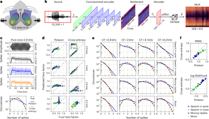
The time-invariant single-branch DNN that was used to predict the neural activity of individual recordings is shown in Fig. 1. The model was trained to map a sound waveform s to neural activity \(\hat\) via an inferred conditional distribution of MUA counts \(p(\hat | s)\) using the following architecture: (1) a SincNet layer³⁶ with 48 bandpass filters of size 64 and stride of 1, followed by a symmetric logarithmic activation \(y=\,\text \,(x)\times \log (| x| +1)\); (2) a stack of five one-dimensional (1D) convolutional layers with 128 filters of size 64 and stride of 2, each followed by a parametric rectified linear unit (PReLU) activation; (3) a 1D bottleneck convolutional layer with 64 filters of size 64 and a stride of 1, followed by a PReLU activation; and (4) a decoder convolutional layer without bias and 512 × N_c filters of size 1, where N_c is the number of parameters in the count distribution \(p({\hat}| s)\) as described below. All convolutional layers in the encoder included a bias term and used a causal kernel. A cropping layer was added after the bottleneck to remove the left context from the output, which eliminated any convolutional edge effects.

For the Poisson model, N_c = 1 and the decoder output was followed by a softplus activation to produce the rate function λ that defined the conditional count distribution for each unit in each time bin (exponential activation was also tested, but softplus yielded better performance). The loss function was \(\mathop{\sum }\nolimits_{m = 1}^{M}\mathop{\sum }\nolimits_{t = 1}^{T}(\lambda [m,t]-R[m,t]\log \lambda [m,t])\), where M and T are the number of units and time bins in the response, respectively. For the cross-entropy model, N_c = 5 and the decoder output was followed by a softmax activation to produce the probability of each possible count n ∈ {0,…, N_c − 1} for each unit in each time bin. The loss function was \(-{\sum }_{m = 1}^{M}{\sum }_{t = 1}^{T}{\sum }_{n = 0}^{{N}_{\mathrm{c}}-1}R[m,t]\log (p(\hat{R}[m,t]=n| s))\). The choice of 4 as the maximum possible count was made on the basis of the MUA count distributions across all datasets (the percentage of counts above 4 was less than 0.02%). All neural activity was clipped during training and inference at a maximum value of 4.

Time-variant single-branch architecture

The time-variant single-branch architecture (Figs. 2 and 3) included an additional time input τ. Each sample of the time input defined the relative time at which the corresponding sound sample was presented during a given recording (range of approximately 0–12 h). To match the dimensionality and dynamic range of the sound input after the SincNet layer, the time input was given to a convolutional layer with 48 filters of size 1 (without bias), followed by a symmetric logarithmic activation. The resulting output was then concatenated to the output of the SincNet layer to form the input of the first convolutional layer of the encoder. The loss function was \(-{\sum }_{m = 1}^{M}{\sum }_{t = 1}^{T}{\sum }_{n = 0}^{{N}_{\mathrm{c}}-1}R[m,t]\log (p(\hat{R}[m,t]=n| s,\tau ))\).

Time-variant multi-branch architecture

The final ICNet model (Figs. 3 and 4) comprises a time-variant DNN with a shared encoder and separate decoder branches for each of the individual animals. The architecture of the encoder and decoders were identical to those in the single-branch models, except for the additional time input. Instead of a single time input to the encoder, a separate time input was used for each animal with the same dimensionality and sampling rate as the bottleneck output. Each sample of the time input thus defined the relative time at which a corresponding MUA sample was recorded and was given to a convolutional layer with 64 filters of size 1 (with bias), followed by a PReLU activation. The output of each of these layers was then multiplied (elementwise) by the bottleneck output and was given to the corresponding decoder.

For the additional analysis in Supplementary Fig. 3, a time-variant multi-branch architecture with a more complex time module was trained. Each time input was given to a cascade of 4 convolutional layers with 128 filters of size 1 (and bias), followed by PReLU activations. The final output of each time module was multiplied by the bottleneck output and given to the corresponding decoder as in the final ICNet.

Linear–nonlinear models

For the comparison of ICNet with linear–nonlinear models in Fig. 3d, single-layer models for seven animals were trained through Poisson regression. The models comprised a convolutional layer with 512 filters (one for each output unit) of size 64 samples and stride 1 (without bias), followed by an exponential activation. Mel spectrograms were used as inputs and were computed as follows: (1) the short-time Fourier transform (STFT) of the audio inputs was computed using a window of 512 samples and a step size of 32 samples, resulting in spectrograms with time resolution of 762.9395 Hz (to match the 1.3-ms time bins of the neural activity); (2) the power spectrograms (squared magnitude of the STFT outputs) were mapped to 96 Mel bands with frequencies logarithmically spaced between 50 Hz and 12 kHz; (3) the logarithm of the Mel spectrograms was computed and was offset by 7 dB so that the spectrograms comprised only positive values; and (4) a sigmoid activation function was applied to normalize the range of the spectrograms. An L2 regularization penalty was additionally applied to the convolutional kernel during training using a factor of 10⁻⁵. A number of parameters for the spectrogram inputs (STFT window size, linear or Mel scale, number of frequency bands, and activation functions) were tested, and the values that produced the best performance were used.

Training

Models were trained to transform 24,414.0625 Hz sound input frames of 8,192 samples into 762.9395 Hz neural activity frames of 256 samples (Fig. 1b). Context of 2,048 samples was added on the left side of the sound input frame (total of 10,240 samples) and was cropped after the bottleneck layer (2,048 divided by a decimation factor of 2⁵ resulted in 64 cropped samples at the level of the bottleneck). Sound inputs were scaled such that a root-mean-square (RMS) value of 0.04 corresponded to a level of 94 dB SPL. For the time-variant models, time inputs were expressed in seconds and were scaled by 1/36,000 to match the dynamic range to that of the sound inputs. These scalings were necessary to enforce training with sufficiently high decimal resolution, while maximally retaining the datasets’ statistical mean close to 0 and standard deviation close to 1 to accelerate training.

The DNN models were trained on NVidia RTX 4090 graphics processing units using Python and Tensorflow³⁷. A batch size of 50 was used with the Adam optimizer and a starting learning rate of 0.0004. All trainings were performed so that the learning rate was halved if the loss in the validation set did not decrease for two consecutive epochs. Early stopping was used and determined the total number of training epochs if the validation loss did not decrease for four consecutive epochs. This resulted in an average of 38.1 ± 3.4 epochs for the nine single-branch models, and a total of 42 epochs for the nine-branch ICNet model. To speed up training, the weights from one of the single-branch models were used to initialize the encoder of the multi-branch models.

Training dataset

All sounds that were used for training the DNN models totalled to 7.83 h and are described below. Ten per cent of the sounds were randomly chosen to form the validation set during training. The order of the sound presentation was randomized for each animal during recording. Multi-branch models were trained using a dataset of 7.05 h, as some of the music sounds were not recorded across all nine animals.

Speech

Sentences were taken from the TIMIT corpus³⁸ that contains speech read by a wide range of American English speakers. The entire corpus excluding ‘SA’ sentences was used and was presented either in quiet or with background noise. The intensity for each sentence was chosen at random from 45, 55, 65, 75, 85 or 95 dB SPL. The SNR was chosen at random from either 0 or 10 when the speech intensity was 55 or 65 dB SPL (as is typical of a quiet setting such as a home or an office) or −10 or 0 when the speech intensity was 75 or 85 dB SPL (as is typical of a noisy setting such as a pub). The total duration of speech in quiet was 1.25 h, and the total duration of speech in noise was 1.58 h.

Noise

Background noise sounds were taken from the Microsoft Scalable Noisy Speech Dataset³⁹, which includes recordings of environmental sounds from a large number of different settings (for example, café, office and roadside) and specific noises (for example, washer–dryer, copy machine and public address announcements). The intensity of the noise presented with each sentence was determined by the intensity of the speech and the SNR as described above.

Processed speech

Speech from the TIMIT corpus was also processed in several ways: (1) the speed was increased by a factor of 2 (via simple resampling without pitch correction of any other additional processing); (2) linear multichannel amplification was applied, with channels centred at 0.5, 1, 2, 4 and 8 kHz and gains of 3, 10, 17, 22 and 25 dB SPL, respectively; or (3) the speed was increased and linear amplification was applied. The total duration of processed speech was 2.08 h.

Music

Pop music was taken from the musdb18 dataset⁴⁰, which contains music in full mixed form as well as in stem form with isolated tracks for drums, bass, vocals and other (for example, guitar and keyboard). The total duration of the music presented from this dataset was 1.28 h. A subportion of this music was used when training multi-branch models, which corresponded to 0.67 h. Classical music was taken from the musopen dataset (https://musopen.org; including piano, violin and orchestral pieces) and was presented either in its original form; after its speed was increased by a factor of 2 or 3; after it was high-pass filtered with a cut-off frequency of 6 kHz; or after its speed was increased and it was high-pass filtered. The total duration of the music presented from this dataset was 0.8 h.

Moving ripples

Dynamic moving ripple sounds were created by modulating a series of sustained sinusoids to achieve a desired distribution of instantaneous amplitude and frequency modulations. The lowest frequency sinusoid was either 300 Hz, 4.7 kHz or 6.2 kHz. The highest-frequency sinusoid was always 10.8 kHz. The series contained sinusoids at frequencies between the lowest and the highest in steps of 0.02 octaves, with the phase of each sinusoid chosen randomly from between 0 and 2π. The modulation envelope was designed so that the instantaneous frequency modulations ranged from 0 to 4 cycles per octave, the instantaneous amplitude modulations ranged from 0 to 10 Hz, and the modulation depth was 50 dB. The total duration of the ripples was 0.67 h.

Abridged training dataset

For the analysis in Fig. 5 (see also Supplementary Figs. 5 and 4), a subportion of all sounds that were described above were used. The abridged training dataset was generated by keeping only the first 180 s of each speech segment (60% of total duration), while preserving the total duration of the remaining sounds. The resulting dataset totalled to 5.78 h (347 min) and included 2.95 h of (processed and unprocessed) speech and 2.83 h of music and ripples. As before, 10% of the sounds were randomly chosen to form the validation set during training.

Evaluation

To predict neural activity using the trained DNN models, the decoder parameters were used to define either a Poisson distribution or a categorical probability distribution with N_c classes using the Tensorflow Probability toolbox⁴¹. The distribution was then sampled from to yield simulated neural activity across time bins and units, as shown in Fig. 1b.

Evaluation dataset

All model evaluations used only sounds that were not part of the training dataset. Each sound segment was 30 s in duration. The timing of the presentation of the evaluation sounds varied across animals. For two animals, each sound was presented only twice and the presentation times were random. For three animals, each sound was presented four times, twice in successive trials during the first half of the recording and twice in successive trials during the second half of the recording. For the other four animals, each sound was presented ten times, twice in successive trials at times that were approximately 20%, 35%, 50%, 65% and 80% of the total recording time, respectively.

Speech in quiet

For all animals, a speech segment from the UCL SCRIBE dataset (http://www.phon.ucl.ac.uk/resource/scribe) consisting of sentences spoken by a male speaker was presented at 60 dB SPL. For four of the animals (Fig. 4b), another speech segment from the same dataset was chosen and was presented at 85 dB SPL, consisting of sentences spoken by a female speaker.

Speech in noise

For all animals, a speech segment from the UCL SCRIBE dataset consisting of sentences spoken by a female speaker was presented at 85 dB SPL in hallway noise from the Microsoft Scalable Noisy Speech Dataset at 0 dB SNR. For four of the animals (Fig. 4b), another speech segment from the same dataset was chosen and was presented at 75 dB SPL, consisting of sentences spoken by a male speaker mixed with café noise from the Microsoft Scalable Noisy Speech Dataset at 4 dB SNR.

Moving ripples

For all animals, dynamic moving ripples with the lowest frequency sinusoid of 4.7 kHz were presented at 85 dB SPL. For four of the animals (Fig. 4b), dynamic moving ripples with the lowest-frequency sinusoid of 300 Hz were also used and were presented at 60 dB SPL.

Music

For all animals, 3 s from each of ten mixed pop songs from the musdb18 dataset were presented at 75 dB SPL. For four of the animals (Fig. 4b), a solo violin recording from the musopen dataset was presented at 85 dB SPL.

Pure tones

For measuring Fano factors (Fig. 1) and assessing systematic errors (Supplementary Fig. 2b), 75-ms tones at four frequencies (891.44, 2,048, 3,565.78 and 8,192 Hz) were presented at either 59 or 85 dB SPL with 10-ms cosine on and off ramps. Each tone was repeated 128 times, and the resulting responses were used to compute the average, the variance and the full distribution of MUA counts (using time bins from 2.5 ms to 80 ms).

Neurophysiological evaluation dataset

For the analysis in Fig. 5 (see also Supplementary Figs. 4 and 5), a dataset was recorded that included sounds commonly used in experimental studies to assess the neurophysiological properties of IC neurons (frequency tuning, temporal dynamics, rate–intensity functions, dynamic range adaptation, forward masking and context enhancement). This evaluation dataset was presented to two animals that were not included in ICNet training, interspersed with sounds from the abridged training dataset described above.

PCA was used to visualize the manifestation of the relevant phenomena in the latent representation of the ICNet bottleneck. PCA was performed separately for each sound, after subtracting the average activity of each bottleneck channel to silence and dividing the resulting responses by −500 (to match the scale and sign of the MUA for plotting).

Frequency tuning

For the results shown in Fig. 5a and Supplementary Figs. 4e and 5a, tones were presented at frequencies from 256 to 16,384 Hz (1/5-octave spacing) and intensities from 4 to 103 dB SPL (9-dB spacing) with 50-ms duration and 10-ms cosine on and off ramps. Each tone was presented eight times in random order with 75 ms of silence between presentations. The responses were used to compute FRA heatmaps by averaging activity across time bins from 7.9 ms to 50 ms after tone onset.

Temporal dynamics

For the results shown in Fig. 5b and Supplementary Fig. 5b, tones were presented at frequencies from 294.1 to 14,263.1 Hz (1/5 octave spacing) and intensities of 59 and 85 dB SPL with 75-ms duration and 10-ms cosine on and off ramps. Each tone was presented 128 times in random order with 75 ms of silence between presentations. The responses were used to compute the average and standard deviation of MUA counts in time bins from 0 to 82.9 ms after tone onset.

Dynamic range adaptation

For the results shown in Fig. 5d and Supplementary Fig. 5d, the sounds defined in ref. ²⁷ were used. For the baseline rate–intensity functions, noise bursts were presented at intensities from 21 to 96 dB SPL (2-dB spacing) with 50-ms duration. Each intensity was presented 32 times in random order with 300 ms of silence between presentations. For the rate–intensity functions of HPR sounds, noise bursts were presented at intensities from 21 to 96 dB SPL (1-dB spacing) with 50-ms duration. The intensities were randomly drawn from a distribution with an HPR of 12 dB range centred at either 39 or 75 dB SPL to create sequences of 16.15 s (no silence was added between noise bursts). Each value in the HPR was drawn 20 times, and all other values were drawn once. Sixteen different random sequences were presented. The responses were used to compute the rate–intensity functions by averaging activity across time bins from 7.9 ms to 50 ms after noise onset.

Amplitude-modulation tuning

For the results shown in Fig. 5c and Supplementary Figs. 4g,h and 5c, the sounds defined in ref. ²⁶ were used. Noise was generated with a duration of 1 s (with 4-ms cosine on and off ramps) and a bandwidth of one octave, centred at frequencies from 500 to 8,000 Hz (1/2-octave spacing). The noise was either unmodulated or modulated with 100% modulation depth at frequencies from 2 to 512 Hz (1-octave spacing). Two different envelope types were used for modulating the noise: a standard sinusoid and a sinusoid raised to the power of 32 (raised-sine-32 envelope in fig. 1a of ref. ²⁶). All sounds were presented six times in random order with 800 ms of silence between presentations.

In an attempt to present the sounds at approximately 30 dB above threshold for most units, each sound was presented at two intensities that varied with centre frequency, with higher intensities used for very low and very high frequencies to account for the higher thresholds at these frequencies. The baseline intensities were 50 and 65 dB SPL with the addition of [15, 0, 0, 0, 20, 20] dB SPL for centre frequencies of [500, 1,000, 2,000, 4,000, 8,000] Hz. The additional intensities for other centre frequencies were determined by interpolating between these values.

To obtain modulation transfer functions, the fast Fourier transform of the responses was computed using time bins from 7.9 ms to 1,007.9 ms after sound onset with a matching number of frequency bins (763 bins). Synchrony was defined as the ratio between the modulation frequency component and the d.c. component (0 Hz) of the magnitude-squared spectrum for all modulation frequencies.

Forward masking

For the results shown in Fig. 5e, Supplementary Figs. 4f and 5e, the sounds defined in ref. ⁴ were used. For the unmasked rate–intensity functions, tones (probes) were presented at frequencies from 500 and 11,313.71 Hz (1/2-octave spacing) with 20-ms duration and 10-ms cosine on and off ramps. The baseline intensities of the tones varied from 5 and 75 dB SPL (5-dB spacing), and the intensity was increased for very low and very high frequencies as described above. Each tone was presented 12 times in random order with 480 ms of silence between tones.

For the masked rate–intensity functions, a masking tone at the same frequency as the probe was presented with a duration of 200 ms and 10-ms cosine on and off ramps, with a 10-ms pause added between the offset of the masker and the onset of the probe. The masker was presented at baseline intensities of 50 and 75 dB SPL, and the intensity was increased for very low and very high frequencies as for the probe tone, but with the additional intensities scaled by 2/3. The responses were used to compute the rate–intensity functions by averaging actvity across time bins from 7.9 ms to 20 ms after probe onset.

Context enhancement

For the results shown in Fig. 5g and Supplementary Fig. 5g, the sounds defined in ref. ²⁹ were used. The conditioner and test sounds were generated by adding together equal-amplitude tonal components with random phases and frequencies from 200 Hz to 16 kHz (1/10-octave spacing). A notch was carved out of the spectrum with centre frequency from 500 to 8,000 Hz (1/2-octave spacing) and width from 0 to 2 octaves (0.5-octave spacing). For the test sound, an additional tone was added at the centre frequency of the notch. The conditioner and test sounds had durations of 500 ms and 100 ms, respectively, with 10-ms cosine on and off ramps. The sounds were presented at baseline intensities of 40 and 60 dB SPL and the intensity was increased for very low and very high frequencies as described above. Each test sound was presented either alone or preceded by the conditioner 12 times in random order with 1.2 s of silence between presentations. The responses were used to compute the average activity across time bins from 7.9 ms to 100 ms after test sound onset.

Non-stationarity

For Fig. 2g, we quantified the non-stationarity in each recording as the absolute difference of the covariance of neural activity elicited by the same sound on two successive trials and on two trials recorded several hours apart. The covariance was computed after flattening (collapsing neural responses across time and units into one dimension). To obtain a single value for the covariance on successive trials, the values from the two pairs of successive trials (one pair from early in the recording and one pair from late in the recording) were averaged. To obtain a single value for the covariance on separated trials, the values from the two pairs of separated trials were averaged.

Overall performance metrics

RMSE and log-likelihood were used as overall performance metrics (Figs. 1–3). The reported results for both metrics were the averages computed over two trials of each sound within each individual recording. One trial was chosen from the first half of the recording and the other from the second, resulting in times of 3.51 ± 1.83 h and 8.92 ± 1.16 h across all nine animals. For each trial, the RMSE and log-likelihood were computed as follows:

where M is the number of units, T is the number of time bins, s is the sound stimulus, τ is the time input, R is the recorded neural activity and \(\hat{R}\) is the predicted neural activity obtained by sampling from the inferred distribution \(p(\hat{R}| s,\tau )\) (or \(p(\hat{R}| s)\) for a time-invariant model).

Predictive power metrics

To assess the predictive power of ICNet (Figs. 2 and 4 and Supplementary Figs. 3 and 4), we selected two metrics that were computed using successive trials for the seven animals for which this was possible (chosen from the beginning of the recording, resulting in times of 1.94 ± 0.46 h across animals). The two metrics are formulated as the fraction of explainable variance or correlation that the model explained across all units. The fraction of explainable correlation explained was computed as follows:

where \({R}_{1},{R}_{2}\in {{\mathbb{N}}}^{M\times T}\) are the recorded neural activity for each trial, \({\hat{R}}_{1},{\hat{R}}_{2}\in {{\mathbb{N}}}^{M\times T}\) are the predicted neural activity and ρ is the correlation coefficient. The responses were flattened (collapsed across time and units into one dimension) before the correlation was computed.

The fraction of explainable variance explained was computed as follows¹⁴:

where E_c denotes expectation over counts of \(p(\hat{R}| s,\tau )\) (or \(p(\hat{R}| s)\) for a time-invariant model). The responses were flattened (collapsed across time and units into one dimension) before the variances in the denominator of equation (4) and in equation (5) were computed, while flattening was achieved in the numerator of equation (4) through the averaging across units and time. To compute the predictive power of ICNet for each unit (Fig. 4d), we computed the formulas of equations (3)–(5) across time only (without collapsing across the unit dimension or averaging across units). Values above 100% for individual units indicate that the ICNet responses were more similar to the recorded responses than the recorded responses were to each other across successive trials, which is possible in recordings with high non-stationarity.

To visualize coherence in Supplementary Fig. 2a, we computed the magnitude-squared coherence for recorded and predicted responses to the four primary evaluation sounds. The coherence of the recorded responses across trials was computed as follows:

where M is the number of units, and G₁₂ is the cross-spectral density between the responses R₁ and R₂ for the two successive trials, while G₁ and G₂ represent the power spectral densities for each of the responses, respectively. The spectral densities were computed across the first dimension of the neural responses (time) using 763 frequency bins and a Hanning window. The coherence of the predicted and recorded responses was obtained by computing the coherence between the predicted and recorded response on each trial using the same formula and taking the average of the two values.

Phoneme recognition

A DNN architecture based on Conv-TasNet⁴² was used to train an ASR back end that predicted phonemes from the ICNet bottleneck response. The DNN architecture comprised: (1) a convolutional layer with 64 filters of size 3 and no bias, followed by a PReLU activation, (2) a normalization layer, followed by a convolutional layer with 128 filters of size 1, (3) a block of 8 dilated convolutional layers (dilation from 1 to 2⁷) with 128 filters of size 3, including PReLU activations and residual skip connections in between, (4) a convolutional layer with 256 filters of size 1, followed by a sigmoid activation, and (5) an output convolutional layer with 40 filters of size 3, followed by a softmax activation. All convolutional layers were 1D and used a causal kernel with a stride of 1.

The ASR model was trained using the train subset of the TIMIT corpus³⁸. The TIMIT sentences were resampled to 24,414.0625 Hz and were segmented into sound input frames of 81,920 samples (windows of 65,536 samples with 50% overlap and left context of 16,384 samples). In each training step, the sound input frames were given to the frozen ICNet model to generate bottleneck responses at 762.9395 Hz (output frames of 2,048 samples with left context of 256 samples). The bottleneck response was then given to the ASR back end to predict the probabilities of the 40 phoneme classes across time (output frames of 2,048 samples at 762.9395 Hz after cropping the context).

The TIMIT sentences were calibrated to randomly selected levels between 40 dB and 90 dB SPL in steps of 5 dB, and were randomly mixed with the 18 noise types from the DEMAND dataset⁴³ at SNRs of −30, −20, −10, 0, 10, 20, 30 and 100 dB. The phonetic transcriptions of the TIMIT dataset were downsampled to the sampling frequency of the neural activity (762.9395 Hz) and were grouped into 40 classes (15 vowels and 24 consonants plus the glottal stop). To account for the phonetic class imbalance (high prevalence of silence in the dataset), a focal cross-entropy loss function was used for training with the focusing parameter γ set to 5.

ASR models were trained to predict speech recognition from the ICNet bottleneck response, as well as from the bottleneck responses of the nine single-branch time-variant models. The trained ASR models were evaluated using six random sentences of the test subset of the TIMIT corpus. The sentences were calibrated at 65 dB SPL, and speech-shaped noise was generated to match the long-term average spectrum of the sentences. A baseline system was also trained with the same DNN architecture, but using a standard Mel spectrogram as the input. The Mel spectrogram was computed from the sound input (24,414.0625 Hz) using frames of 512 samples, a hop size of 32 samples and 64 Mel channels with frequencies logarithmically spaced from 50 to 12,000 Hz. These parameters were chosen to maximize performance while matching the resolution of the ICNet bottleneck response (762.9395 Hz output frames with 64 channels).

Statistics

Confidence intervals for all reported values were computed using 1,000 bootstrap samples. For the metrics that we used to assess model performance (RMSE, log-likelihood, variance and correlation explained), bootstrapping was performed across units for each animal. For the ASR results (Fig. 3f), bootstrapping was performed across animals.