InstaNovo enables diffusion-powered de novo peptide sequencing in large-scale proteomics experiments

1 14 minutes read

InstaNovo enables diffusion powered de novo peptide sequencing in large scale proteomics.png

Data

Training dataset retrieval and preparation

IN was trained on the large-scale ProteomeTools³⁶ dataset, which has been recorded with modern, state-of-the-art instrumentation, containing high-resolution spectra for peptides of human origin. This dataset comprises over 700,000 synthetic tryptic peptides covering the entirety of canonical human proteins and isoforms, as well as encompassing peptides generated from alternative proteases and HLA peptides. We used the data from the first three parts of the ProteomeTools project, and split the database search results into two datasets. The first dataset is derived from the evidence results of the MaxQuant⁶¹ searches available in the repository, and contains the highest-confidence PSMs per peptide and is therefore referred to as the HC-PT dataset. The second dataset contains all PSMs regardless of quality (derived from the MS results of the searches), and is referred to as the AC-PT dataset. The HC-PT dataset contains 2.6 million unique spectra, and the unfiltered AC-PT dataset contains 28 million total spectra. Both datasets contain 742,000 unique peptides (Fig. 1a). Distributions of the dataset properties show expected behaviour in terms of m/z, charge, measurement error and so on (Extended Data Fig. 1). After obtaining the training data from the repository, we devised a pipeline to extract the spectrum information and associated metadata we believed were needed for model training (Fig. 1b and Supplementary Fig. 1).

In more detail, to ensure a consistent analysis, only the 3x high-energy collision-induced dissociation (HCD) data were utilized, as they provided an inclusion list and employed 3 different HCD fragmentation energies. The raw data files were converted to mzML format using the Proteowizard MSConvert tool⁶², with default settings. The result files obtained from MaxQuant⁶¹ (‘evidence.txt’ or ‘msms.txt’ for high-confidence or full dataset, respectively) were employed to extract scan indices for identified peptides, as well as the associated metadata (precursor mass, charge, measurement error, retention time) for each PSM. To facilitate further analysis, the pyOpenMS Python⁶³ wrapper of the OpenMS C library was utilized. This tool enabled the reading of mzML files, extraction of scans and association of the scans with the PSM metadata. To refine the dataset and set a padding threshold for the model input features, PSMs were filtered based on specific criteria. Only peptides with a length of 30 or fewer residues and a maximum of 800 peaks in the spectrum were included in the analysis. In all of our experiments, we used residues with the following PTMs: carbamidomethylation for cysteine, oxidation for methionine, and deamidation for asparagine and glutamine.

Data splits

We did a 80:10:10 train/validation/test split for HC-PT and AC-PT based on the unique peptide sequences. When splitting, we ensured that there was no leakage between the HC-PT sets and the AC-PT sets (that is, no HC-PT train samples are present in the AC-PT test set, and so on). All models and hyperparameters were chosen based on their validation set performance. Test-set results were computed only when writing up the paper and used for the reported figures. All results shown in the paper are reported on the test set. For yeast, bacillus and mouse, we used the splits as defined in DeepNovo³⁰ and PointNovo⁴⁸.

Model implementations

Development of InstaNovo architecture

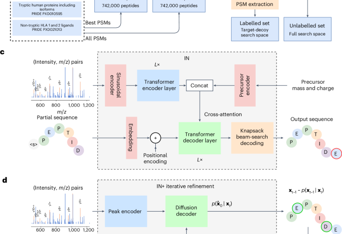
The IN architecture is based on the transformer encoder–decoder architecture⁶⁴. Similar to PointNovo⁴⁸ and Casanovo²⁹, we represent our MS2 spectra as the set of N peaks (m, I), where m = m₁, m₂, …, m_N and I = I₁, I₂, …, I_N represent the sets of m/z and intensity, respectively. To encode these peaks, we employ multi-scale sinusoidal embeddings³³. We process these encoded peaks through a transformer encoder layer, allowing the model to self-attend and extract relative information between the peaks. The encoder output is concatenated with a learnt latent spectrum and a representation of the encoding of the precursor. The precursor mass m_prec and charge c_prec are encoded with a sinusoidal encoding and embedding layer, respectively, after which they are summed to represent the precursor embedding. This precursor may alternatively be encoded as the start-of-sequence token in the decoder, but we found no difference to model performance. The encoder has 9 layers, each with 16 heads, a hidden dimension of 768, and a feed-forward dimension of 1,024. This encoder allows the fragment ions and their intensities to self-attend to other ions present in the spectrum.

The transformer decoder, also consisting of 9 layers with 16 heads each, makes use of causal autoregressive decoding. This enables the model to take in the previous residues from the predicted sequence and autoregressively predict the next token. The partially decoded sequence is encoded through an embedding layer and a standard sinusoidal positional encoding is added. The input sequence is automatically prepended with a start-of-sequence token. The decoder cross-attends over the encoder output, latent spectra and precursor encoding.

For the causal autoregressive decoding, we implement knapsack beam search decoding. This eliminates the need for multiple predictions and retains performance while increasing model confidence and decreasing FDRs in the full search space. IN recall is marginally reduced across datasets (0.05–0.2%) compared with a standard beam search with 5 predictions per spectrum, and peptide inference takes longer compared with beam search, but reductions in almost all error types justify its use.

IN has 95 million parameters in total. To train IN, we implement the model in PyTorch⁶⁵, with PyTorch Lightning⁶⁶ being used to handle the training loop. The loss function computes the cross-entropy between the predicted model logits and the ground-truth peptide. All training and model hyperparameters are provided in Supplementary Table 1.

Iterative refinement with InstaNovo+

After our initial model training and promising results in sequence decoding, we speculated that next-token prediction is not the most optimal approach to mass spectrum sequence decoding.

Under HCD and collision-induced dissociation fragmentation, the most intense ions are the b and y ions^67,68,69,70 of the peptide, with the y ions of tryptic peptides generally having better readout properties, potentially due to charge localization. For that reason, many de novo sequencing models start token prediction from the right-hand side of the sequence, as we also do for our base model IN. However, we argued that as internal y or even b ions are more intense, there might be an advantage in exploring approaches that decode the peptide sequence all at once instead of performing next-token prediction (Supplementary Fig. 5).

Hence, in addition to IN, we introduce IN+, based on a similar transformer architecture but with a different goal. Rather than autoregressive decoding, the IN+ model is trained to perform multinomial diffusion^47,71. This means the model is trained to iteratively remove noise from a corrupted sequence (see Supplementary Note 2 for further details). The full model architecture is given in Supplementary Fig. 2b.

When decoding IN+, we decode five samples for each spectrum. The sequence that matches the precursor mass with the highest log probability under the model is selected as the IN+ prediction. In the case where we start with an IN prediction and none of the IN+ predictions satisfy the precursor mass, we instead fall back to the IN prediction used at t = 15 (which should always fit the precursor).

Metrics and benchmarks

We use peptide recall as our main benchmarking metric for testing and validation datasets. As this is the more stringent of metrics used in de novo sequencing algorithm evaluation, we believe that this metric reflects our model’s performance the best. We also report peptide precision, as well as amino acid residue precision, recall and error rates for our training and validation datasets. We formulate our metrics as done in ref. ⁴⁹ (see Supplementary Note 4 for details). We further compared our models with baselines using the entire receiver operating characteristic curve rather than just the precision and recall at a single confidence threshold. We obtained these by varying the confidence threshold from the highest to the lowest values obtained in an evaluation dataset and plotting the resulting pairs of (amino acid or peptide level) precisions and recall values.

We decoded peptides from our models using beam search with knapsack filtering (Supplementary Note 5, Algorithm 1). This ensured that the system always found a peptide that fit the precursor mass, improving overall performance and reducing the frequency of almost all individual error types. Beam search (with beam width B) is a variant of breadth-first search where at each step, the frontier is pruned to the B highest scoring sequences. We use knapsack filtering in beam search to allow only amino acid sequences that can be continued so that their theoretical mass matches the precursor mass to a 50 ppm relative difference. See Supplementary Note 5 for further details.

Application-oriented datasets

Nanobodies

The nanobodies included in this study (Supplementary Table 2) were discovered using phage display technology (see Supplementary Note 9 for further details). The nanobody concentration was determined by measuring the absorbance at 280 nm in a NanoDrop One (ThermoFisher Scientific). From each stock solution, 10 μg of nanobody was transferred, the buffer was exchanged and the volume was reduced with SP3 bead clean-up⁷² and following on-bead digestion. In brief, pure ethanol was added to a final concentration of 80%. Fifty micrograms of each hydrophobic and hydrophilic beads (Cytiva, Sera-Mag Carboxylate-Modified [E7] Magnetic Particles 24152105050250 and Sera-Mag SpeedBead Carboxylate-Modified [E3] Magnetic Particles 65152105050250) were added to the solution, and incubated in a thermomixer at room temperature, at 800 rpm, for 15 min to allow binding. Samples were placed in a magnetic rack and the solvent was removed. The remaining beads and bound proteins were washed 3 times with 90% ethanol, and were finally resuspended in 20 μl of 2.5 M guanidine hydrochloride (GuHCl; G3272 Sigma-Aldrich) and 250 mM HEPES solution (4-(2-hydroxyethyl)piperazine-1-ethanesulfonic acid; 7365-45-9 Sigma-Aldrich). Nanobodies were reduced and alkylated with 10 mM TCEP (tris(3-hydroxypropyl triazolyl methyl)amine; 762342 Sigma-Aldrich) and 40 mM CAA (2-chloroacetamide; 79-07-2 Sigma-Aldrich), incubated for 10 min at 95 °C. Samples were diluted 5 times in MilliQ water, and 200 ng trypsin (V5280 Promega Gold) was added to a 1:50 protease:proteome ratio, assuming no losses. Samples were digested overnight, at 37 °C, 450 rpm. The next day, samples were placed on a magnetic rack and the solution was transferred to a new tube. Approximately 500 ng of peptides, assuming no losses, was acidified and loaded on EvoTips with the standard loading protocol⁷³ for MS analysis. The samples were analysed using the EvoSep One liquid chromatography platform, in line with an Orbitrap Exploris 480 mass spectrometer equipped with a FAIMSpro device.

Peptides were separated with a PepSep C18 column (15 cm × 75 μm, 1.9 μm PepSep, 1893473), over 31 min, employing the Whisper100 40SPD method. Peptides were ionized with nanospray ionization with a 10 μm emitter (PepSep, 1893527), and spray voltage of 2,300 V in positive-ion mode, and ion transfer tube of 240 °C. The total carrier gas flow was set to 3.6 l min⁻¹, and FAIMS was operated at standard acquisition. Spectra were acquired in data-dependent resolution mode, under two different compensation voltages of −50 and −70 V, with identical settings. The cycle time was set to 2 s, with MS1 spectra acquired with 60,000 resolution, a scan range of 375–1,500, a normalized AGC target of 300%, a radio-frequency lens of 40% and an automatic injection time. Filters were set for peptide MIPS mode, inclusion of charge states 2–6, dynamic exclusion of 60 s with 10 ppm tolerance and an intensity threshold of 10,000. MS2 spectra were acquired with an isolation window of 1.6 m/z, normalized HCD of 30%, Orbitrap resolution of 30,000, first mass at 120 m/z, normalized AGC target of 100% and an automatic injection time. Data analysis was performed in Proteome Discoverer⁷⁴ v2.4, with Sequest HT⁷⁵ as the search engine. The database used was the E. coli reference proteome (Uniprot reviewed, UP000284592, 4,360 sequences, accessed 1 December 2022) concatenated with the nanobody sequences, and additional dynamic modifications of acetylation or methionine loss at the protein N-terminus, along with methionine oxidation, and static modification of carbamidomethylation. FDR control was performed with Percolator, at 1% and 5% target FDRs. Precursor quantification was performed with the Minora Feature Detector and Feature Mapper nodes in the processing and consensus workflows, respectively. Abundances were based on unique and razor peptides and above a signal-to-noise ratio of 5, and normalized based on total protein amount. PSMs at 1% FDR were exported for further processing, data extraction and model validation.

HeLa proteome

HeLa cells were cultured in T25 flasks with Dulbecco’s modified Eagle medium (10565018, ThermoFisher Scientific) until confluency. Cells were pelleted with centrifugation, and resuspended in 6 M GuHCl. Proteins were reduced, alkylated and digested as for nanobodies above, with an additional LysC digestion for 1 h at 1:100 protease:protein ratio, before tryptic digestion. Two-hundred nanograms of peptides, assuming no losses, were acidified and analysed with a nLC E1200 in line with an Orbitrap Exploris 480 mass spectrometer equipped with a FAIMSpro device. Peptides were separated with an 15 cm × 75 μm, 2 μm EASY-SpayTM column (ThermoFisher Scientific, ES904) over a 70 min gradient, starting at 6% buffer B (80% acetonitrile, 0.1% formic acid), increasing to 23% for 43 min, then to 38% for 12 min, 60% for 5 min, 95% for 3 min, and staying at 95% for 7 min. Peptides were ionized with electrospray ionization with a positive-ion spray voltage of 2,000 V, and ion transfer tube of 275 °C. The rest of the method settings were as described above, with the difference of top-20 data-dependent scans, and normalized HCD of 28% for MS2 spectrum acquisition. Data analysis was performed as above, with the only differences being the use of human database (Uniprot reviewed, UP000005640, 20,518 sequences, accessed 5 March 2023), and lack of normalization of precursor quantification in the consensus workflow.

‘Candidatus Scalindua brodae’ proteome

Cells were pelleted and lysed under native conditions with hypotonic buffer (10 mM HEPES, 10 mM NaCl, 1.5 mM MgCl₂, 2 mM EDTA, 0.1% NP-40, Roche Mini protease inhibitor) and a probe sonicator (20% power, 10 s with 1 s pulse, 5 rounds) on ice. Lysates were upconcentrated and buffer exchanged with spin filters (Amicon, 3 kDa cut-off, UFC500324, Merck Millipore) to 50 mM HEPES pH 7.8, and their concentration was determined by Nanodrop. From then on, the standard proteomics sample preparation was followed, starting with 50 μg of proteome. Proteins were reduced, alkylated and digested as described above. Assuming no losses, 1 μg of peptides was acidified and loaded on EvoTips with the low-input protocol. The samples were analysed with EvoSep One liquid chromatography platform, in line with an Orbitrap Eclipse mass spectrometer equipped with a FAIMSpro device. Peptides were separated with a PepSep C18 15 cm × 150 μm, 1.9 μm (PepSep, 1893471), over 44 min with the standard 30SPD method. Peptides were ionized with nanospray ionization with an 10 μm emitter (PepSep, 1893527), and spray voltage of 2,300 V in positive-ion mode, and ion transfer tube of 240 °C. Spectra were acquired in data-dependent acquisition mode, under 2 different compensation voltages of −50 and −70 V, with identical settings. The cycle time was set to 1.2 s, with MS1 spectra acquired with 60,000 resolution, and a maximum injection time of 118 s. MS2 spectra were acquired with an isolation window of 1.6 m/z, normalized HCD of 30%, with otherwise similar settings as above. Data analysis was performed as above, with the only differences being the use of the putative proteome ‘Candidatus Scalindua brodae’ database, assembled from metagenomics data (Uniprot Trembl, UP000030652, 4,014 sequences, accessed 28 February 2023), and lack of normalization of precursor quantification in the consensus workflow. In a secondary search, the raw data were searched against the ‘Candidatus Scalindua brodae’ proteome as above, along with the proteomes of Candidatus Kuenenia stuttgartiensis (UP000221734, 3,801 sequences, accessed 27 July 2023), Candidatus Scalindua rubra (UP000094056, 5,207 sequences, accessed 27 July 2023) and the Candidatus Scalindua profunda metagenome from a previous study (23,834 sequences)⁷⁶.

GluC degradome and PRM monitoring

HeLa cell lysates were extracted as in the HeLa proteome section. Six aliquots of 20 μg of lysate were resuspended in 100 mM HEPES, pH 7.8 to reduce the GuHCl concentration to 0.5 M. Two-hundred nanograms of GluC endopeptidase (V1651, Promega) was added to 3 out of the 6 samples to a protease to proteome ratio of 1:100 ratio, and all samples were incubated at 37 °C, 450 rpm, for 20 min. Samples were reduced, alkylated and digested with trypsin as described previously. The next day, volume equivalent to 1 μg from each sample, assuming no losses, was loaded on EvoTips as described above, and samples were analysed using the EvoSep One liquid chromatography platform, in line with an Orbitrap Eclipse mass spectrometer equipped with a FAIMSpro device. Peptides were eluted from a PepSep C18 column (15 cm × 75 μm, 1.9 μm PepSep, 1893473) over 58 min with the Whisper100 20SPD method. Scans were acquired with the same settings as in the HeLa proteome single-shot analysis. Data analysis was performed as above, with use of the human database for the HeLa proteome searches, semi-tryptic search and precursor quantification normalized on the total peptide amount from each sample in the consensus workflow.

PRM assays were designed for representative peptides detected by IN with high confidence, but not with the database search. Peptide sequences were imported in Skyline⁷⁷, and an inclusion list with the precursor masses was exported. The inclusion list was used to create a PRM monitoring method with a targeted mass inclusion filter for acquisition of MS/MS scans. GluC degradome samples were analysed with the same set-up as in shotgun proteomics and the same FAIMS compensation voltages. Scans were acquired with 60,000 resolution for MS1 and 15,000 resolution for MS2, and a cycle time of 1 s for each FAIMS compensation voltage, with otherwise similar settings with the shotgun proteomics experiment. Results were analysed and visualized with Skyline.

Wound exudate pathogen validation

The wound exudates were extracted from patient wound dressings as described in ref. ⁵⁰. PCR amplification of the 16S rRNA gene was performed using MyTaq Red Mix (Bioline) in a final reaction volume of 20 μl, with 2 sets of primers: 1 specific for the 16S rRNA gene of E. coli (expected amplicon size 544 bp; annealing temperature 60 °C)⁷⁸ and another specific for the 16S rRNA gene of Pseudomonas spp. (expected amplicon size 544 bp; T_m 54 °C)⁷⁹. Each reaction contained 10 μl of MyTaq Red Mix, 1 μl of each primer, 2 μl of the sample, and nuclease-free water to adjust the final volume. As positive controls, 1 μl of a colony dilution prepared from fresh colonies of E. coli BL21(DE3) or P. aeruginosa PA01 was used. PCR was conducted with an initial denaturation at 95 °C for 3 min, followed by 35 cycles of 95 °C for 20 s, annealing at the primer-specific T_m (60 °C or 54 °C) for 20 s (Supplementary Table 3), and extension at 72 °C for 20 s, with a final extension at 72 °C for 90 s. Post-PCR, 6 μl of each reaction product was loaded onto a 1% (w/v) agarose gel prepared in 1X TAE buffer containing SYBR Safe (S33102, ThermoFisher). Electrophoresis was carried out at 100 V for 45 min, and DNA bands were visualized under ultraviolet light using a gel documentation system, with a 1 kb Plus DNA ladder (ThermoFisher) as the molecular weight reference.

External dataset analysis

The raw data from a snake venom proteomics dataset were downloaded and reanalysed using the Uniprot database sequences for the serpentes order (331,759 sequences, accessed 5 September 2022), similar to the original study. Data were analysed with Proteome Discoverer v2.4 and the Sequest HT search engine, with all files included in the same analysis, normalization on total peptide amount and precursor quantification, with other settings similar to other datasets. The herceptin dataset was downloaded and analysed similarly. However, the raw data from the six different proteases were searched separately, and no precursor or normalization was performed. The same fasta database as in the original study was used for PSM detection. Search results were then combined for prediction and evaluation.

The immunopeptidomics dataset was reprocessed with the same proteome database as in the original paper with MSFragger¹³ and the FragPipe v21.1 pipeline with the non-specific HLA workflow, and otherwise default settings. MSBooster⁸⁰ was used for rescoring with deep learning prediction, and Percolator was used for PSM FDR control, while no FDR control was used on the protein level.

The wound fluid dataset was downloaded and searched with the same human database as used for the HeLa proteome and GluC degradomics experiments. Both raw data files were analysed in the same search in Proteome Discoverer v2.4, with total peptide amount normalization and precursor quantification. In the secondary search results, the same human proteome as well as protein sequences downloaded from the Uniprot database for the pathogens of interest Citrobacter sp. (UP000682339, 3,414 sequences), P. aeruginosa (UP000002438, 5,564 sequences), S. aureus (UP000008816, 2,889 sequences) and E. coli (UP000000625, 4,403 sequences) were used for PSM detection.