NYC City Council speaker Adrienne Adams running for mayor

Former New York Gov. is facing a new Democratic challenger in his bid to replace Eric Adams as New York City Mayor, according to reports. 

New York City Council Speaker Adrienne Adams, 64, will officially launch her campaign with a rally over the weekend, per reporting from . 

With the Democratic primary just four months away, Adams is expected to immediately petition to secure ballot access. 

In a statement to media outlets, Adams said New Yorkers couldn’t afford to live in the city, that City Hall was “in chaos,” and alleged that President Donald Trump was “.” 

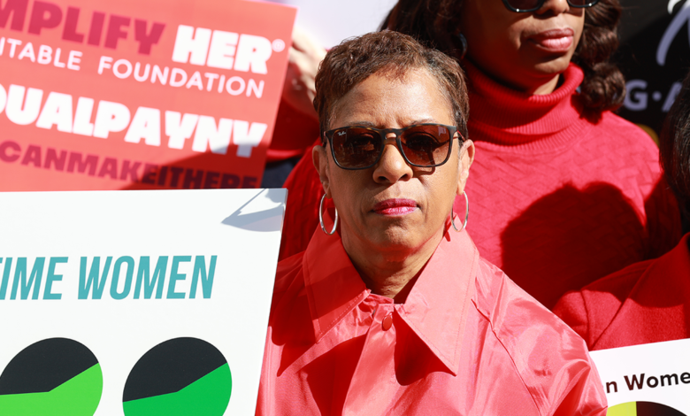
New York City Council Speaker Adrienne Adams launches run to replace incumbent Mayor Eric Adams, challenging the front-runner, former New York Gov. Andrew Cuomo. (Luiz C. Ribeiro for NY Daily News via Getty Images)

“It’s time to stand up. I never planned to run for Mayor, but I’m not giving up on New York City,” Adams said in the statement, first shared with Politico. 

First elected to the city council in 2017, Adams went on to become the first Black council speaker five years later. 

City Council Speaker Adrienne Adams during rally on the steps of New York City Hall before convening the entire Council to vote and override Mayor Adams’ veto of the “How Many Stops Act” on Jan. 30, 2024.  (New York Daily News for NY Daily News via Getty Images)

Adams is the latest high-profile figure to throw her hat in the ring, challenging the front-runner, former New York Gov. Andrew Cuomo, to replace embattled NYC Mayor Eric Adams. 

Cuomo resigned in 2021 after a report released by the state attorney general concluded that he had sexually harassed nearly a dozen women.

New York City Council Speaker Adrienne Adams speaks during a press conference before a New York City Council meeting at City Hall in Manhattan, New York, in December 2023. (Shawn Inglima for NY Daily News via Getty Images)

Cuomo has apologized for having “offended” the women with remarks he said were intended to be collegial, and admitted that he had sometimes been “too familiar” with people, but he denied touching anyone inappropriately and said the investigation of his conduct was flawed and politically motivated.

The race comes after was indicted in September on federal corruption charges. He is now dealing with a tempest of criticism after Trump’s newly installed Justice Department leaders asked a court to drop the case, so Adams could assist with the federal government’s immigration crackdown.

Fox News Digital has reached out to Speaker Adams’ office for comment. 

The Associated Press contributed to this report.